Advanced Tutorial: Thermal Comfort In a Meeting Room

This article provides a step-by-step tutorial for the full thermal comfort assessment in a meeting room using CFD simulation, including models for conjugate heat transfer, radiation/solar load heat transfer, and age of air.

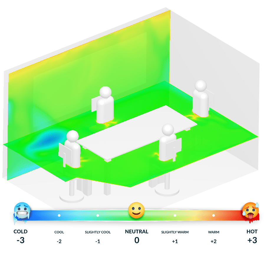
Overview

This tutorial teaches how to:

• Set up and run a conjugate heat transfer flow simulation
• Assign boundary conditions, material, and other models to the simulation
• Mesh the geometry with the SimScale standard meshing algorithm
• Set up result controls for local mean age of air computation
• Set up radiation and solar load heat transfer
• Define thermal comfort parameters computation.

The typical SimScale workflow will be followed:

1. Prepare the CAD model for the simulation.
2. Set up the simulation.
3. Set up the mesh.
4. Run the simulation and analyze the results.

1. Prepare the CAD Model and Select the Analysis Type

First of all, click the button below. It will copy the tutorial project containing the geometry into your own Workbench.

The following picture demonstrates what should be visible after importing the tutorial project.

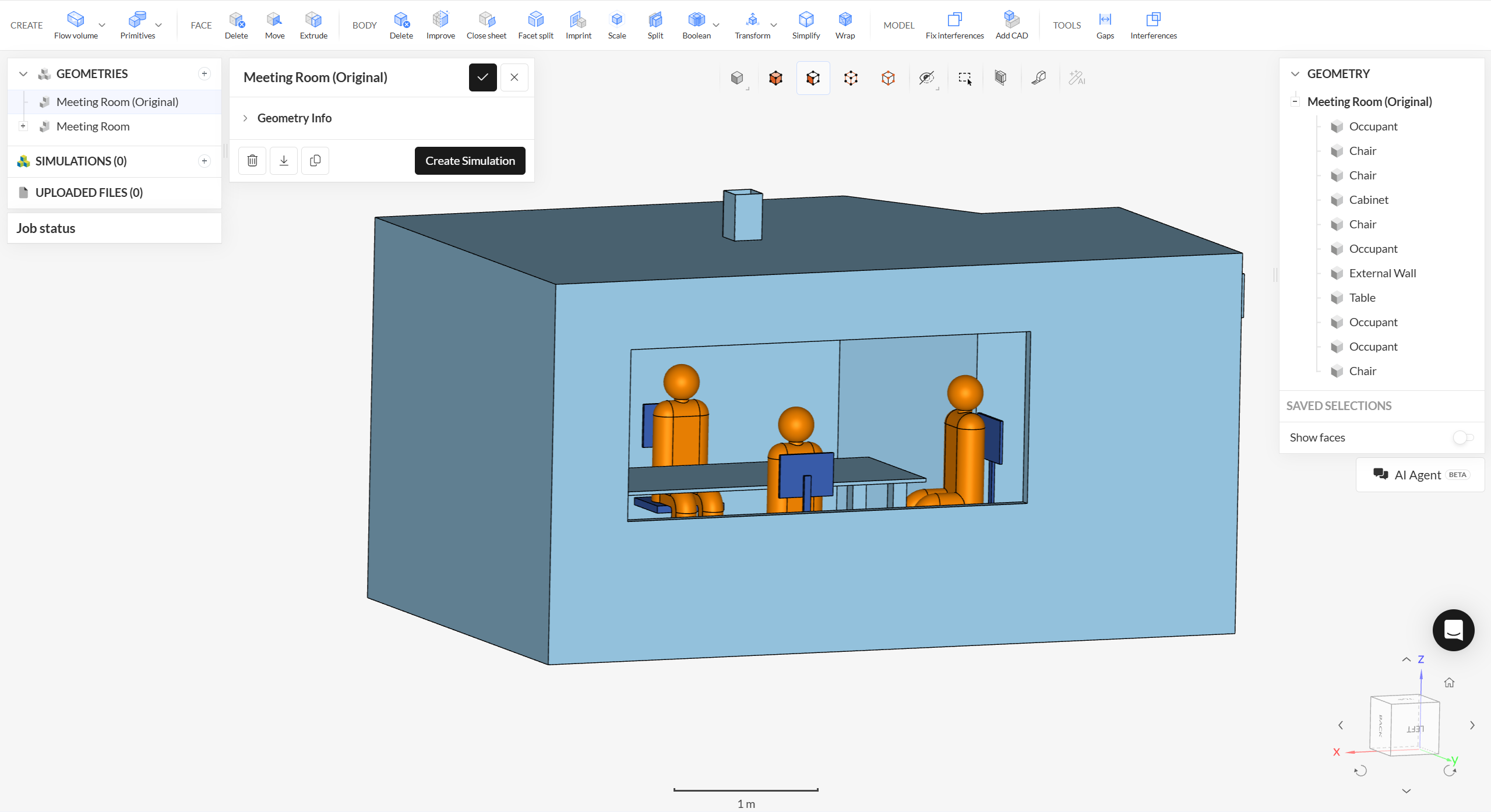
Please notice that the imported project contains two geometries: Meeting Room (Original), containing the solid parts of the domain but no flow region. The second volume, which will be used in the rest of this tutorial, named Meeting Room, contains the flow region that represents the volume of air inside of the room, which must be used in the setup of the simulation.

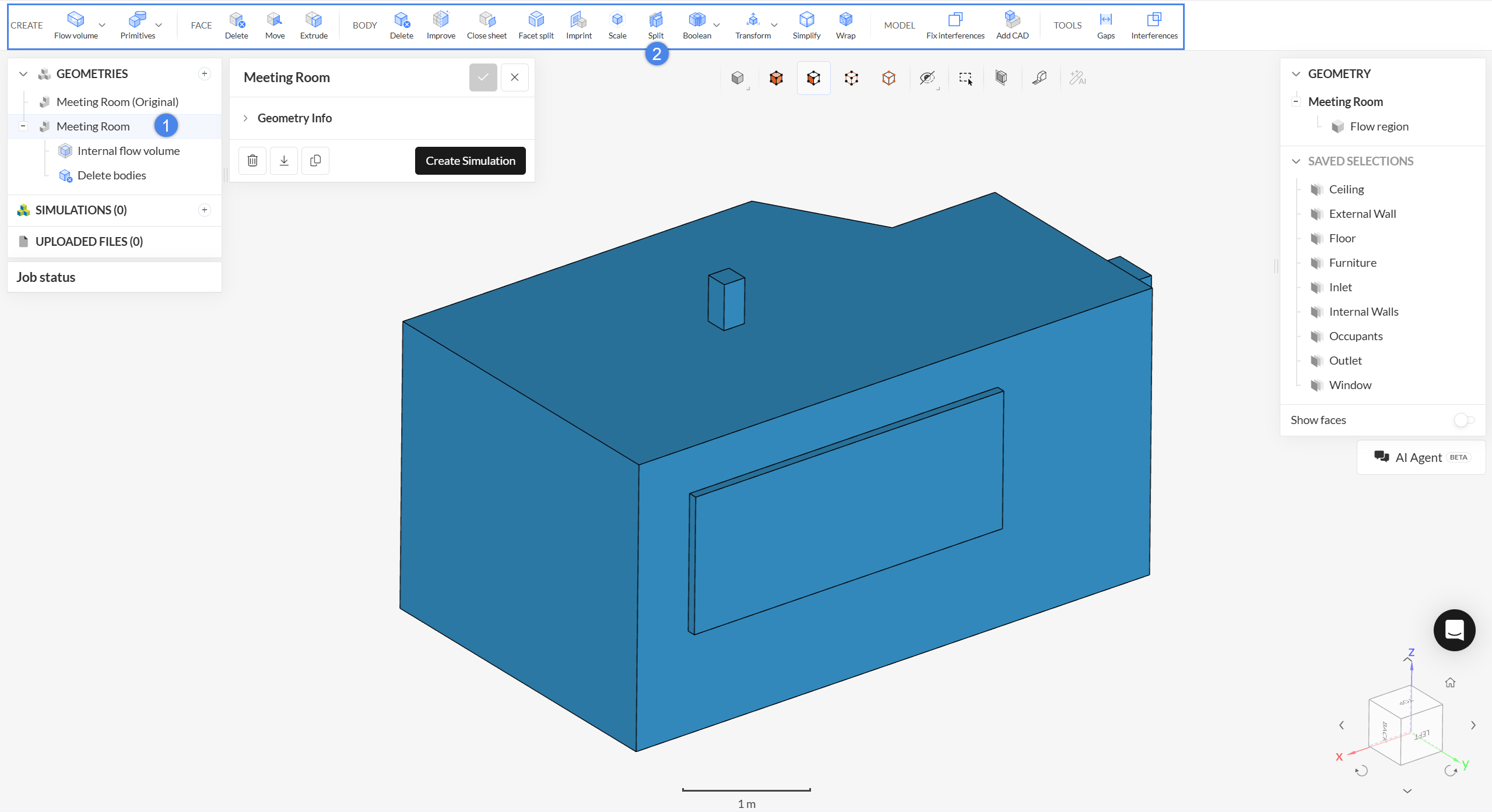
The flow region was already created with an Internal flow volume operation in the CAD editing environment. Note how this volume of air represents the negative of the room and everything inside. In SimScale, you may make changes to the CAD model from the CAD editing environment. To modify a CAD model, simply select the geometry from the list—the available CAD operations will then appear in the top toolbar. You can either work directly on the original model or create a duplicate and apply your changes to the copy.

1.1 Create Saved Selections

Saved selections are groups of faces created at this point to be used in assignments for boundary conditions and other concepts, during the simulation setup. While saved selections are not necessary for the setup of a simulation in SimScale, they can speed up the simulation setup at times. Saved selections can be found at the right-hand side panel:

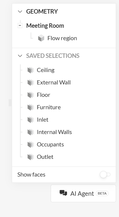
A number of sets are already provided in the project, but one set for the window is still missing. The picture below shows how to add the missing saved selection:

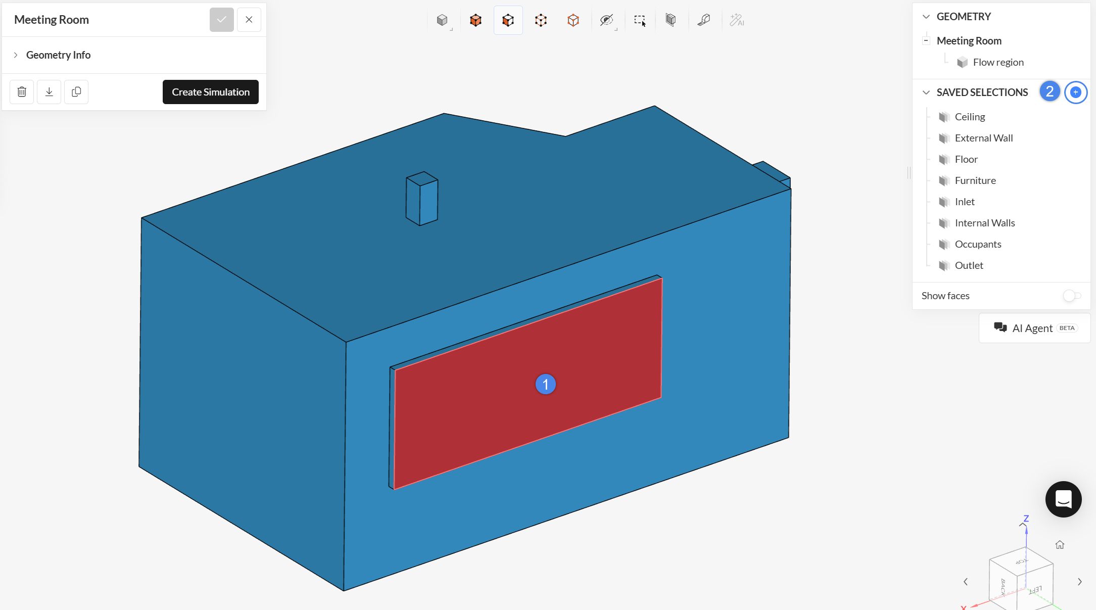
1. Create saved selections by selecting the Window face (highlighted in red),
2. Then click on the ‘+’ icon next to Saved Selections in the right panel.

In the pop-up dialog that appears, name the set “Window” and click ‘Create new selection‘.

1.2 Create the Simulation

Now we can start with the simulation setup. Follow the steps presented in the picture below to create a new simulation:

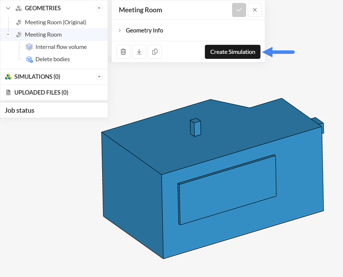
1. Select the ‘Meeting Room’ geometry from the left panel,
2. then click the ‘Create Simulation’ button of the dialog:

The simulation library window appears:

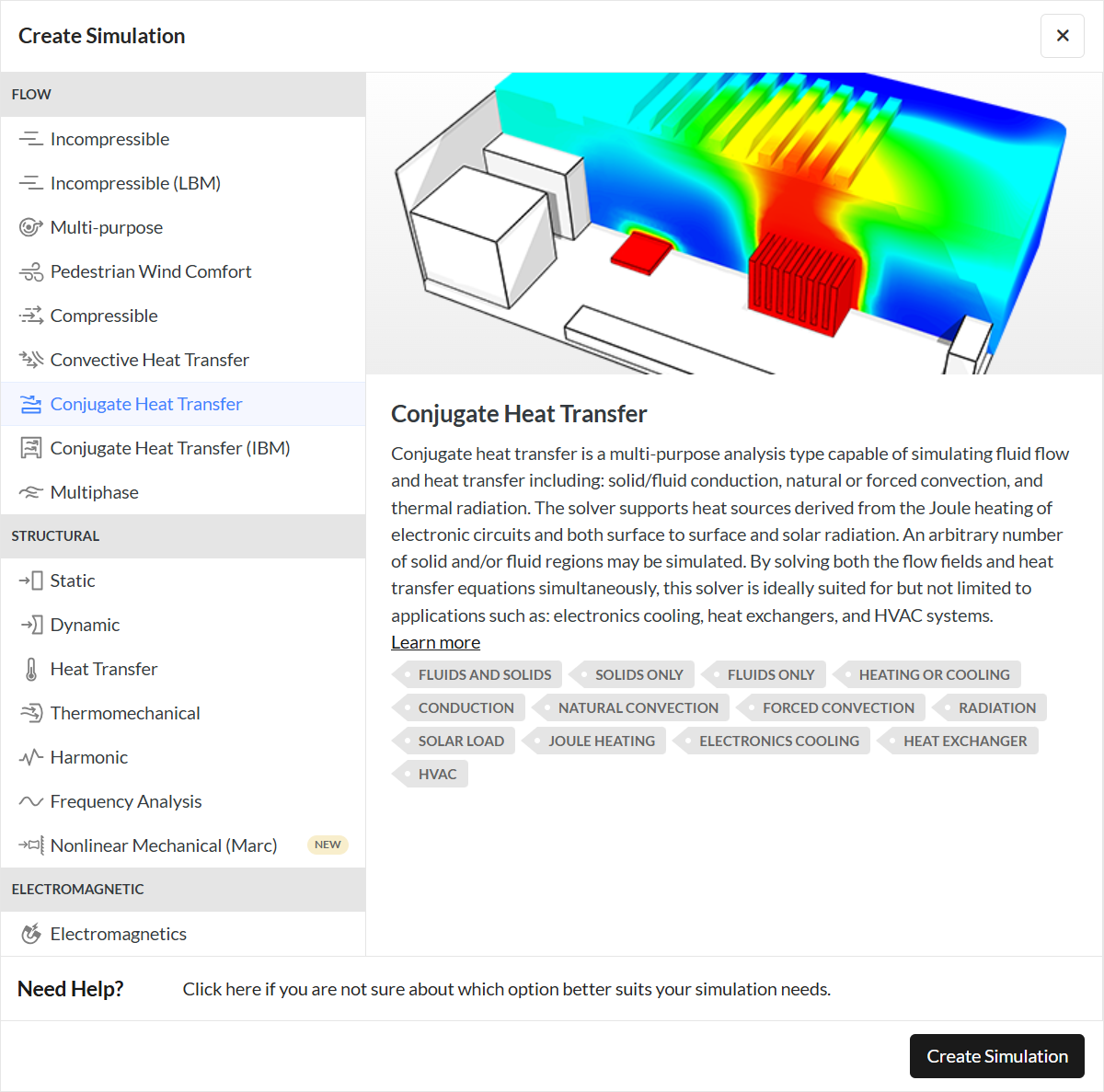
Here you can select the analysis type you need.

• Choose ‘Conjugate Heat Transfer’ and click on ‘Create Simulation‘.
• Now, you will see a new simulation tree element with it’s default settings dialog open:

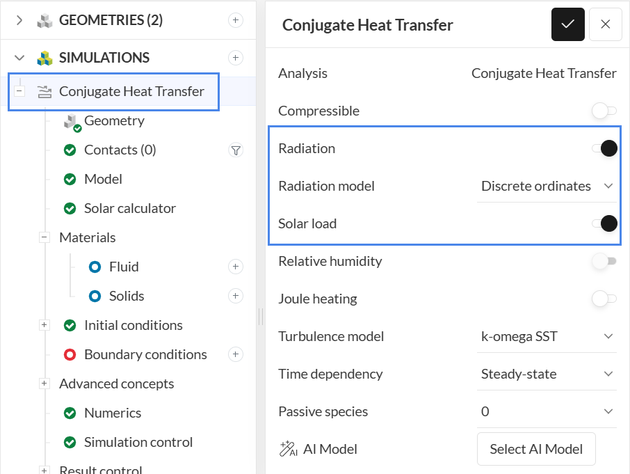
• Activate Solar load and Radiation for the simulation.

Do not forget to click the checkmark at the top to save the changes.

2. Set up the Simulation

In order to have an overview, the following is a description of the simulation model and conditions:

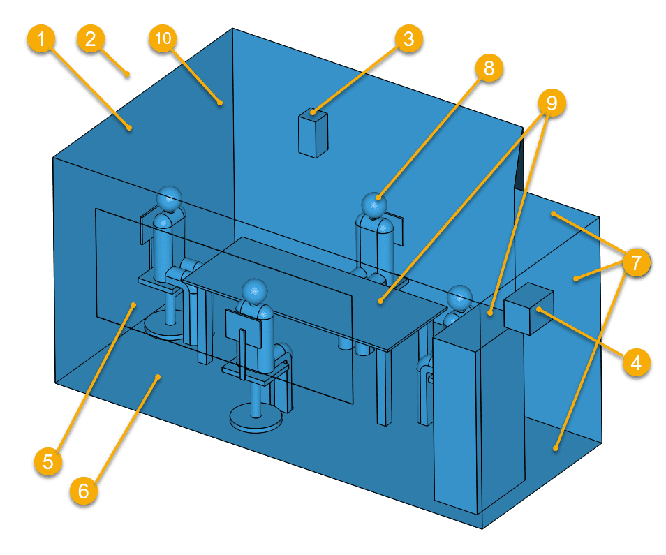
1. Heat transfer is performed through convection, solar load, and radiation
2. Conditions for summer with an ambient temperature of 30 \(°C\) and relative humidity of 65%
3. Outlet flow at the top duct
4. The inlet flow rate of 0.1 \(m^3/s\) and 18 \(°C\) at the side duct
5. Window, which will be closed for the first scenario
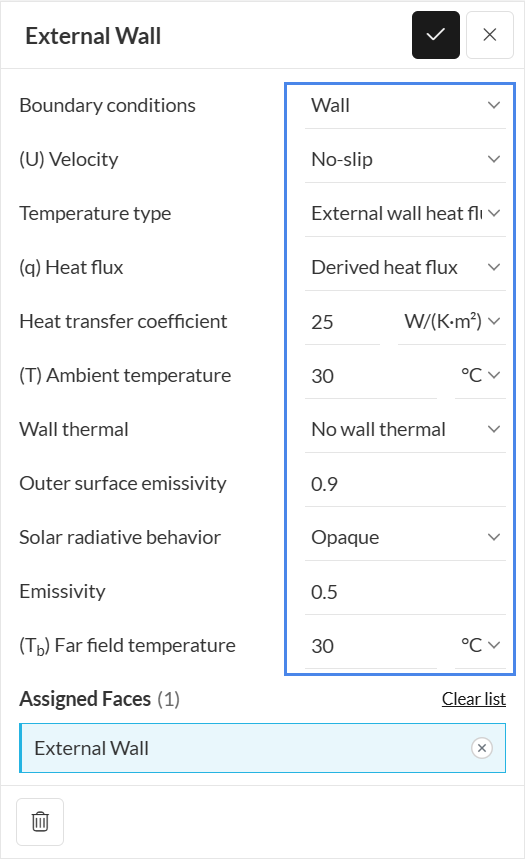
6. Conductive walls to an external temperature of 30 \(°C\) for the external walls
7. Adiabatic walls for the ceiling and floor. Internal walls will exchange heat with the neighboring rooms
8. Flux power heat source of 40.79 \(W/m^2\) for the occupants’ metabolic rate
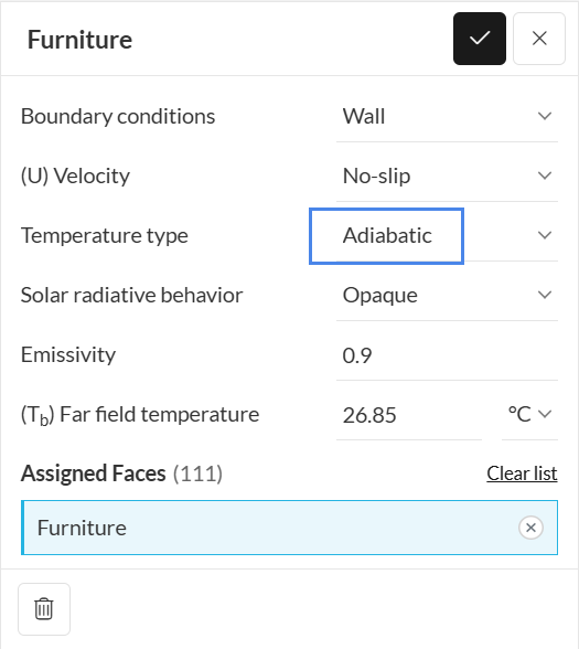
9. Adiabatic walls for the furniture
10. The age of air is modeled through the local mean age of fluid result control

You can explore the corresponding faces for each condition by clicking the saved selections at the right panel.

2.1 Model

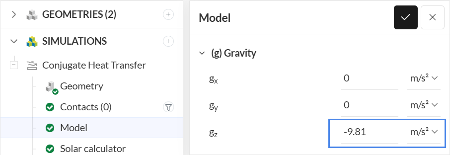
Select the Model tree element to specify the gravitational acceleration. In this tutorial, gravity will be ‘-9.81’ \(m/s^2\) in the z direction.

2.2 Solar Calculator

The solar calculator panel allows you to define the Sun direction and the direct and diffuse Solar load configuration. In this tutorial we will use custom definitions for both, as below:

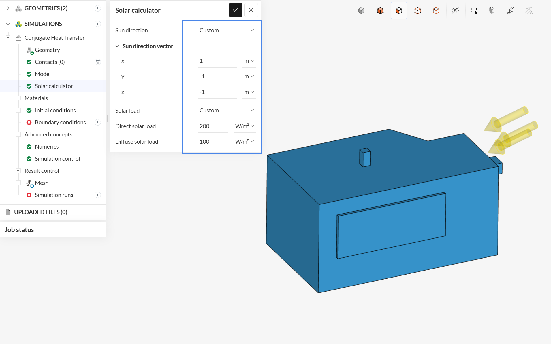
The sun direction is:

• ‘1’ in X
• ‘-1’ in Y
• ‘-1’ in Z

Furthermore, the Direct solar load is ‘200’ \(W/m^2\) and the Diffuse solar load is ‘100’ \(W/m^2\).

2.2 Material

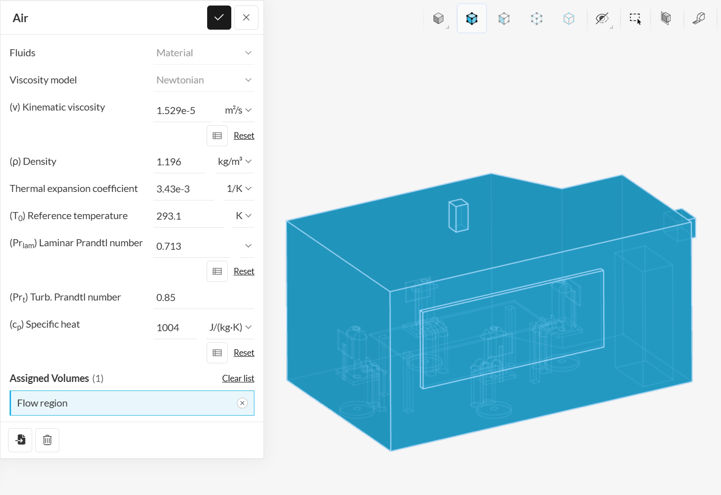
To define and assign a material, please click on ‘+’ next to Materials. Doing so, the SimScale material library will pop up:

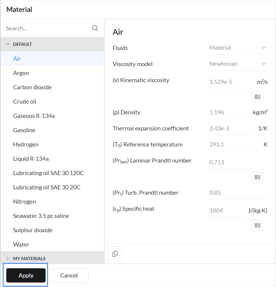
1. Select ‘Air’ from the materials library and click ‘Apply’.
2. As the CAD model contains just one volume, air is automatically assigned to it
3. Accept the selection with the check mark button.

2.3 Boundary Conditions

Now we need to set up the boundary conditions presented in Figure 10. Note that there are two versions of the setup:

1. Forced convection: The ventilation system provides airflow within the room and the window is considered to be closed.
2. Natural convection: The ventilation system does not provide airflow and the window is considered to be open.

We will start with the settings necessary for both scenarios, and then move to the scenario-specific settings.

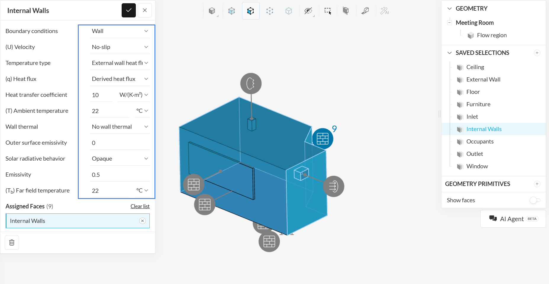
a. Internal Walls

Internal walls are assigned as a ‘Wall’ boundary condition, and as they are facing the inside of the building, they are considered adiabatic.

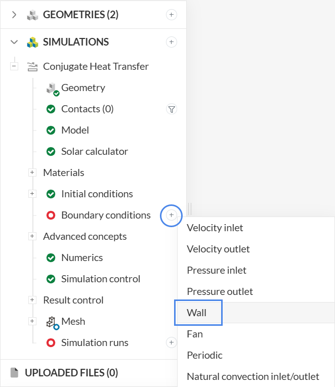
Create a ‘Wall’ boundary condition and assign the Internal Wall saved selection. Set up the parameters as shown in the reference picture:

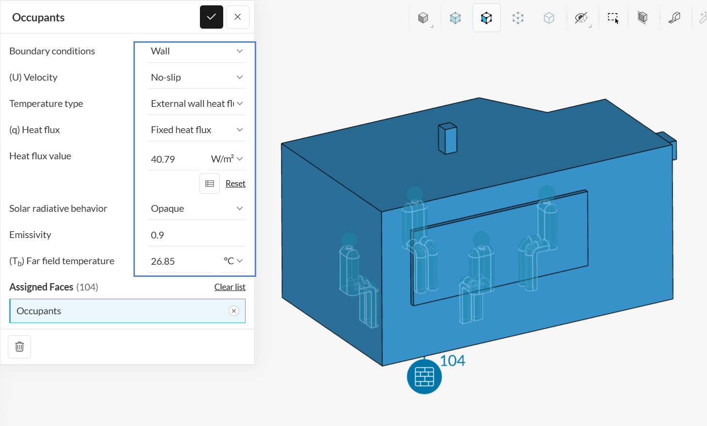
b. Occupants

For the occupants, a wall boundary condition is also used, this time with a heat flux power source to model the metabolic heat generation rate. Create a ‘Wall’ boundary condition and assign the Occupants set. Set up the parameters as shown in the picture:

c. Furniture

For the furniture, a wall boundary condition is also used, with adiabatic thermal behavior. Create a ‘Wall’ boundary condition and assign the Furniture set. Set up the parameters as shown in the picture:

d. External Wall

For the external wall, a wall boundary condition is also used, with a thermal wall model and convection to the exterior. Create a ‘Wall’ boundary condition and assign the External Wall saved selection. Set up the parameters as shown in the picture:

As far as inlet goes, this tutorial offers two options: you can add a natural convection setup to simulate a model without air conditioning where the window is open for natural cooling, or a forced convection setup to simulate the scenario when the window is closed and the air conditioning is on.

Version 1: Cooling with Forced Convection Boundary Conditions

a. Flow Inlet

For the first version of the setup, involving forced convection, the inlet will receive a ‘Velocity inlet’ boundary condition.

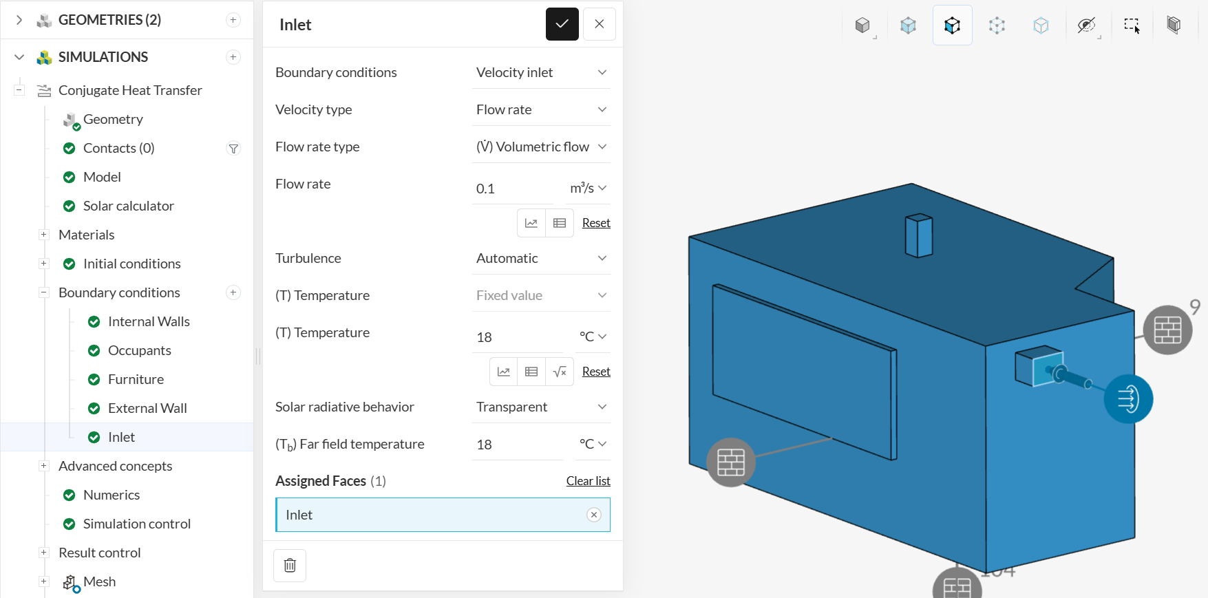
Please modify the following:

• Set a Volumetric flow rate of ‘0.1’ \(m^3/s\),
• Temperature and Far field temperature of ’18’ \(°C\),
• For the assignment, select the ‘Inlet’ face. You can find it as the predefined Inlet saved selections in the geometry tree on the right side of the Workbench.

b. Flow Outlet

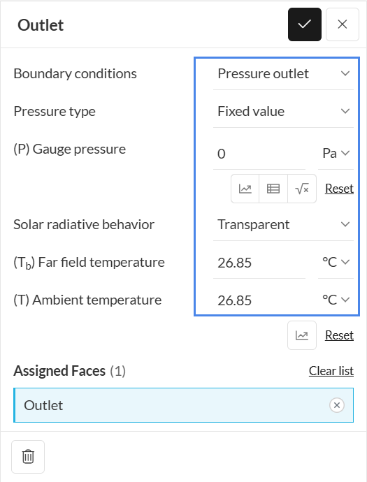
For the flow outlet boundary condition, follow the same procedure, but select a ‘Pressure outlet’. Leave all values as default and assign the Outlet set, as shown in the image:

c. Closed Window

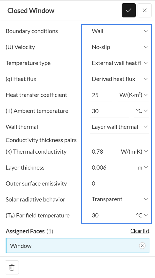
For the window, a wall boundary condition is also used, but this time with a layer wall thermal model, convection to the exterior temperature, and an external radiation source to model sunlight. Create a ‘Wall’ boundary condition and assign the Window set. Set up the parameters as shown in the image:

Version 2: Cooling with Natural Convection Boundary Conditions

a. Natural Convection Inlet/Outlet

For the second version, instead of defining inlets, outlets, and the closed window as indicated in the previous section, all three saved selections will be assigned to a ‘Natural convection inlet/outlet’ boundary condition instead.

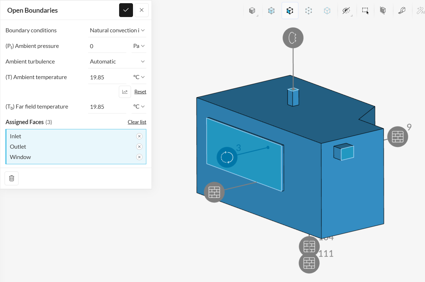
With a natural convection inlet/outlet boundary condition, fluid may go in or out through the boundary, which represents an open path.

2.4 Numerics and Simulation Control

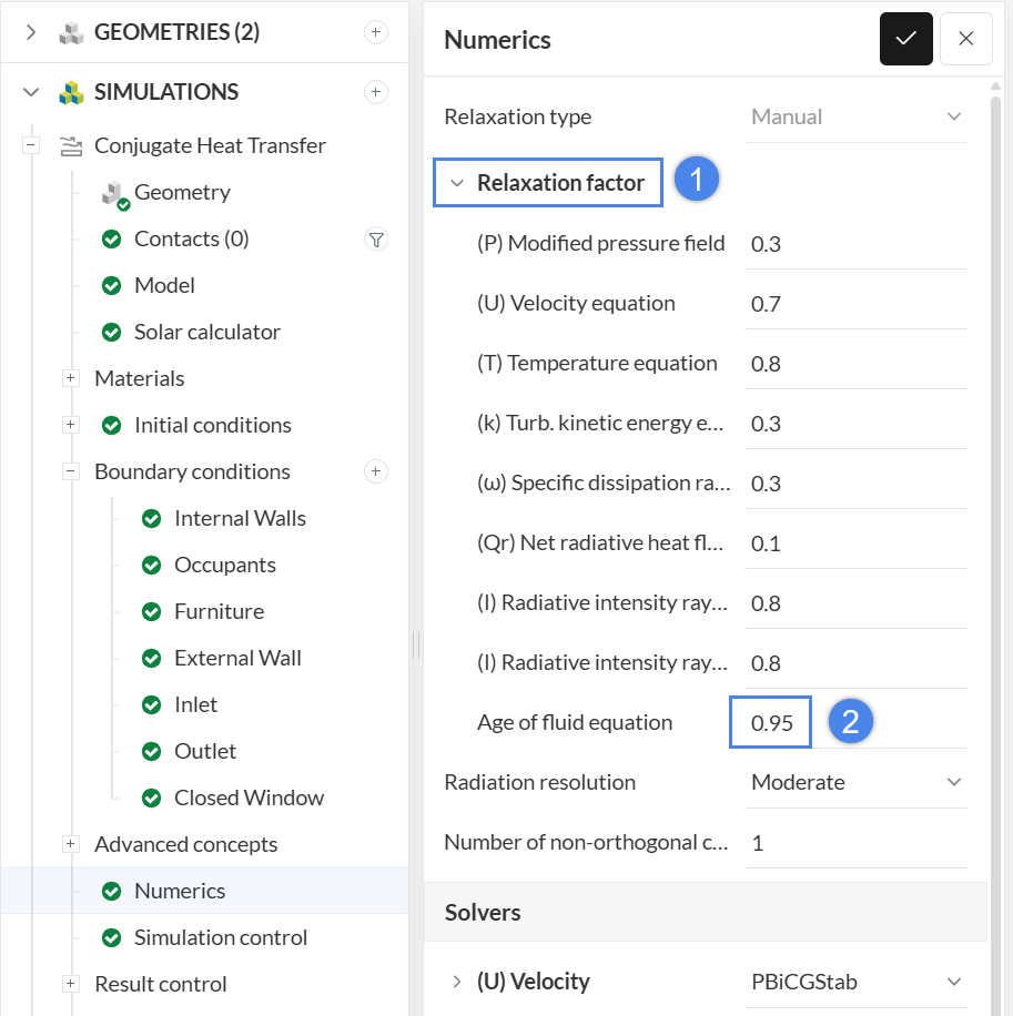
Simulation control, will retain default settings. For Numerics, please adjust the relaxation factor of Age of fluid equation to ‘0.95’.

2.5 Result Control Items

Result control items are used to retrieve specific computations from the numerical solver. By using them, we can have a look at specific variables at specific regions by querying the computation and output of our quantities of interest.

a. Mean Age of Fluid

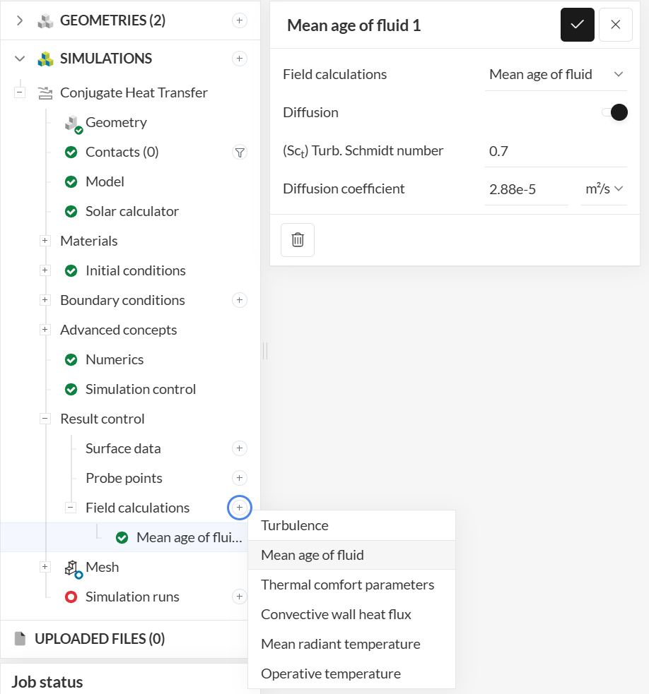
In order to measure the mean age of air in the domain, a Result control item is used. It is created as shown in the picture:

To monitor the age of fluid at the outlet, it is a good idea to create an ‘Area average’ result control within Surface data.

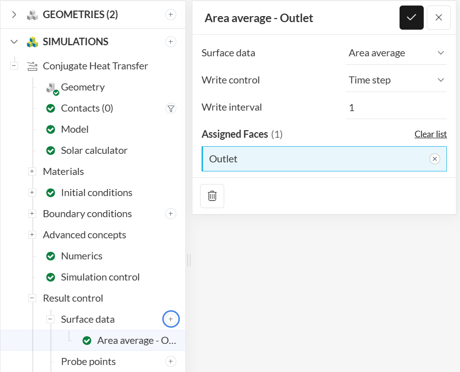
1. Click the ‘+’ icon next to Surface data,
2. Select ‘Area average’ and assign the outlet face

b. Thermal Comfort Parameters

Thermal comfort parameters are also queried in the result control items, under Field calculations. Create the concept as shown in the picture:

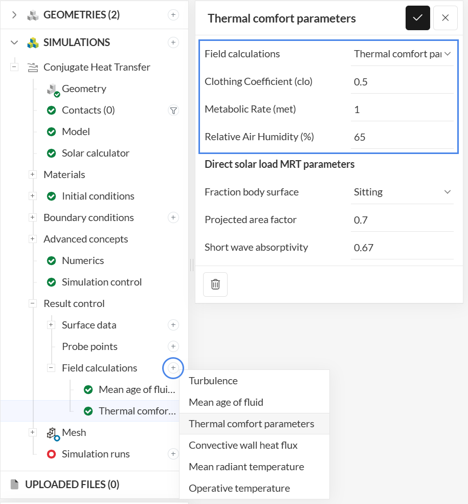
Set up the parameters as shown in the picture:

• In this case, the Clothing coefficient is ‘0.5’,
• the Metabolic rate is ‘1’,
• and the Relative air humidity (%) is ‘65%’.

A description of the computed quantities and resulting fields can be found on this SimScale documentation page: Thermal Comfort Parameters.

3. Mesh

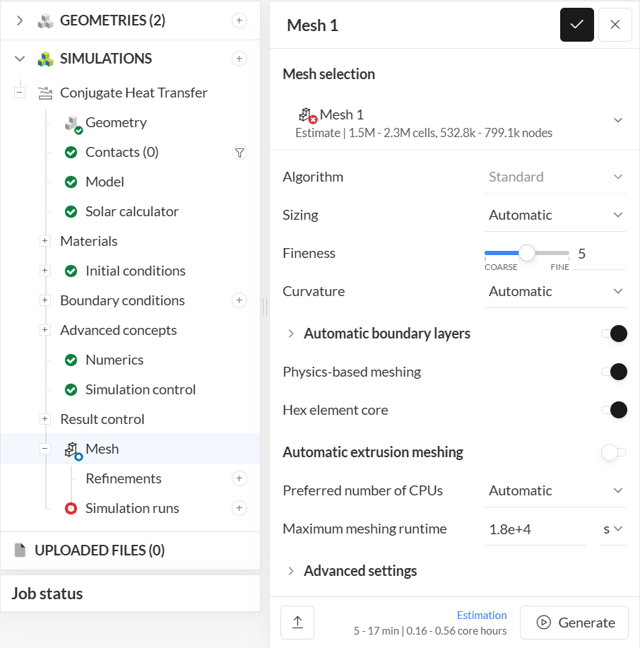
The mesh will stay with default settings for this tutorial. You do not need to click Generate, as the mesh will be computed as part of the simulation run.

4. Start the Simulation

Now that the simulation setup is complete, a new ‘Simulation Run’ can be created to perform the computation. In the following picture, the whole tree setup is shown, and the item to create the simulation run is highlighted:

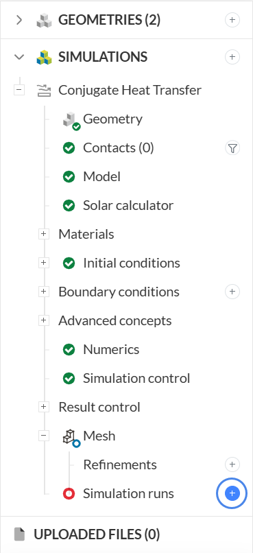
In the pop-up window, press ‘Run anyway’ in case any warning messages appear. This will start the meshing operation and then the simulation immediately. If the software predicts a higher duration of simulation and exceeding maximum runtime you can choose to ignore it or go back to simulation control settings and increase the maximum runtime value.

The computation takes around one and a half hours to complete. If you can’t wait to see the results, at the end of the article there is a link to the completed version of the project.

5. Post-Processing

We will use the integrated post-processor to visualize the temperature inside the meeting room, evaluate the thermal comfort of the room by visualizing the Percentage Mean Vote (PMV), and the local mean age of the air. You may access the post-processor by clicking on the ‘Solution Fields’ button.

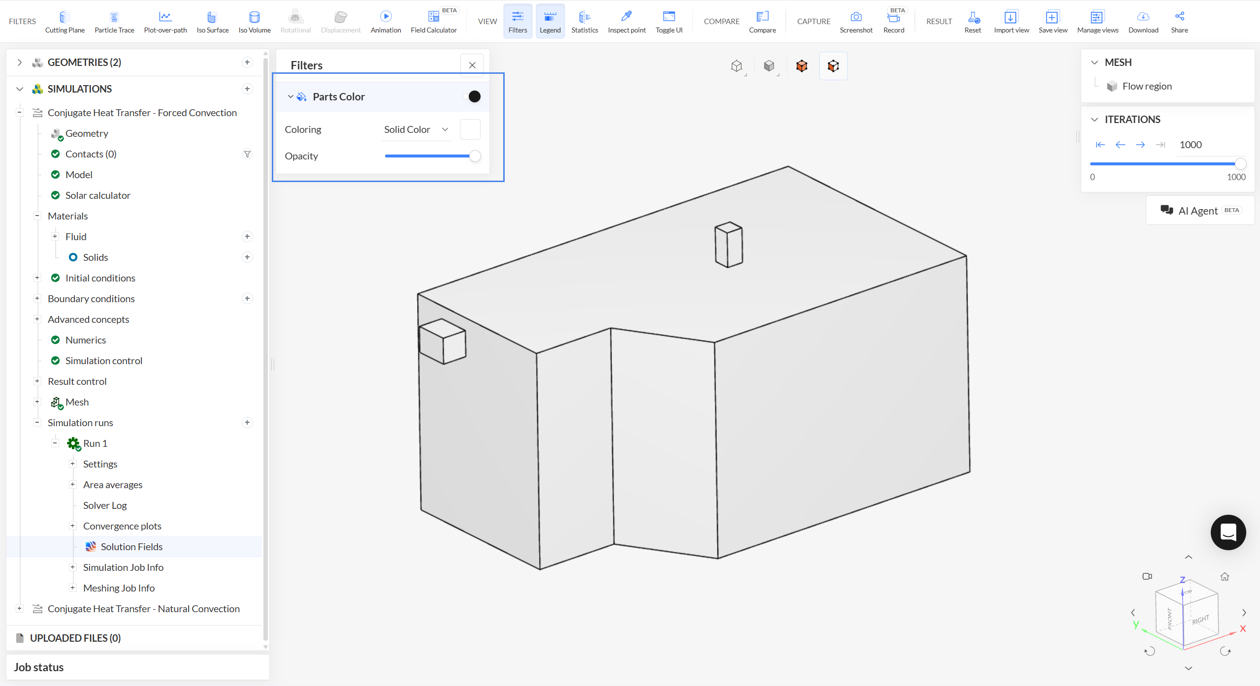
Before starting to post-process the results, make sure that there are no predefined filters. You can delete existing filters at any time by clicking on the dustbin icon next to them. Furthermore, please ensure that you are at the last timestep of your simulation by sliding the Iterations selector all the way to the right.

5.1 Temperature

Visualize the temperature by selecting ‘Temperature’ as the Coloring for your parts. Change the units of temperature to Celsius by clicking the units in the legend and selecting ‘°C’ and change the maximum temperature visualized to ’40’ \(°C\). Hide the walls of the room by selecting them and right-clicking on your mouse to select ‘Hide selection’. The temperature distribution inside the room can be seen in the figure below:

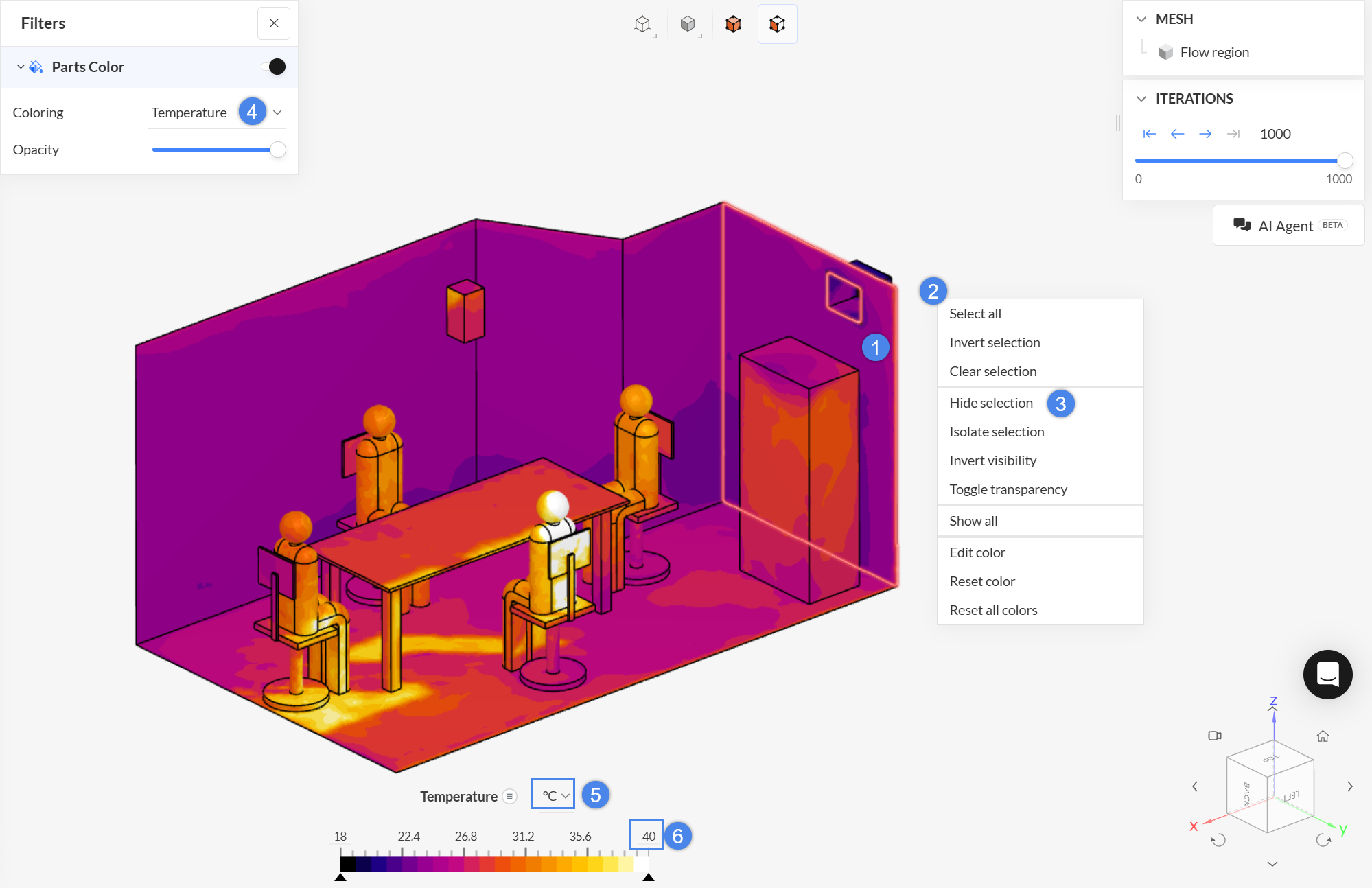
From the figure above, it’s possible to notice the effect of the solar load that goes through the window. The room is unevenly heated with the floor being slightly cool to neutral as we progress towards the ceiling where it is slightly warm.

5.2 Predicted Mean Vote (PMV)

Next, we will focus on visualizing the thermal comfort parameters, which are the predicted mean vote (PMV) and predicted percentage dissatisfied (PPD). The thermal comfort parameters will be visualized by using the cutting plane filter. Follow the steps below to create a cutting plane:

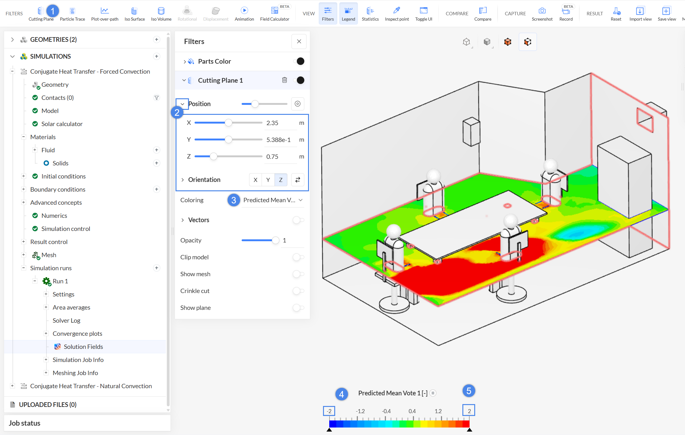
1. Select ‘Cutting plane’ from the top ribbon to create a new filter
2. Configure the cutting plane, so that it is placed at the mid-height of the room. Adjust the Position of the cutting plane by using the following coordinates: ‘2.35, 0.5, 0.75’. The Orientation of the cutting plane should be in the ‘Z’ axis
3. Change the Coloring to the ‘Predicted Mean Vote’. Disable the Clip model slider, so that the model is not clipped
4. Adjust the minimum and maximum PMV legend bounds if needed

Using the same approach from above, create a second cutting plane normal to the ‘Y’ axis. The predicted mean vote (PMV) thermal comfort index distribution is displayed in the following picture:

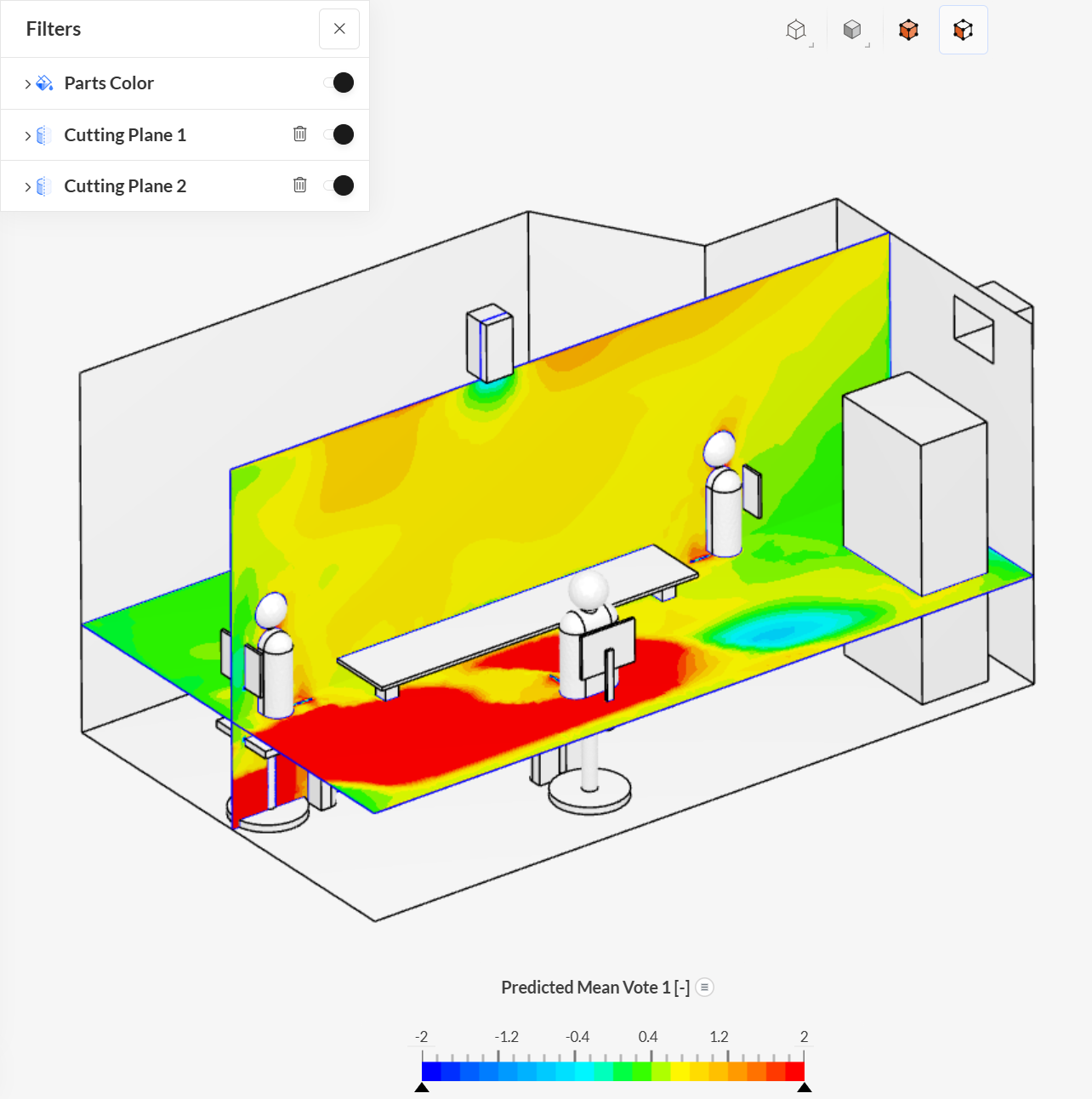
The value of the index is clipped to the recommended range of [-2, 2]. This way, we can visualize the areas that are below and above them, with blue and red colored regions respectively.

5.3 Local Mean Age (LMA) of Air

You can access the age of air results in the post-processor by selecting Mean age of fluid for the filters. The Local Mean Age (LMA) was computed at around 330 seconds at the outlet for the forced convection scenario:

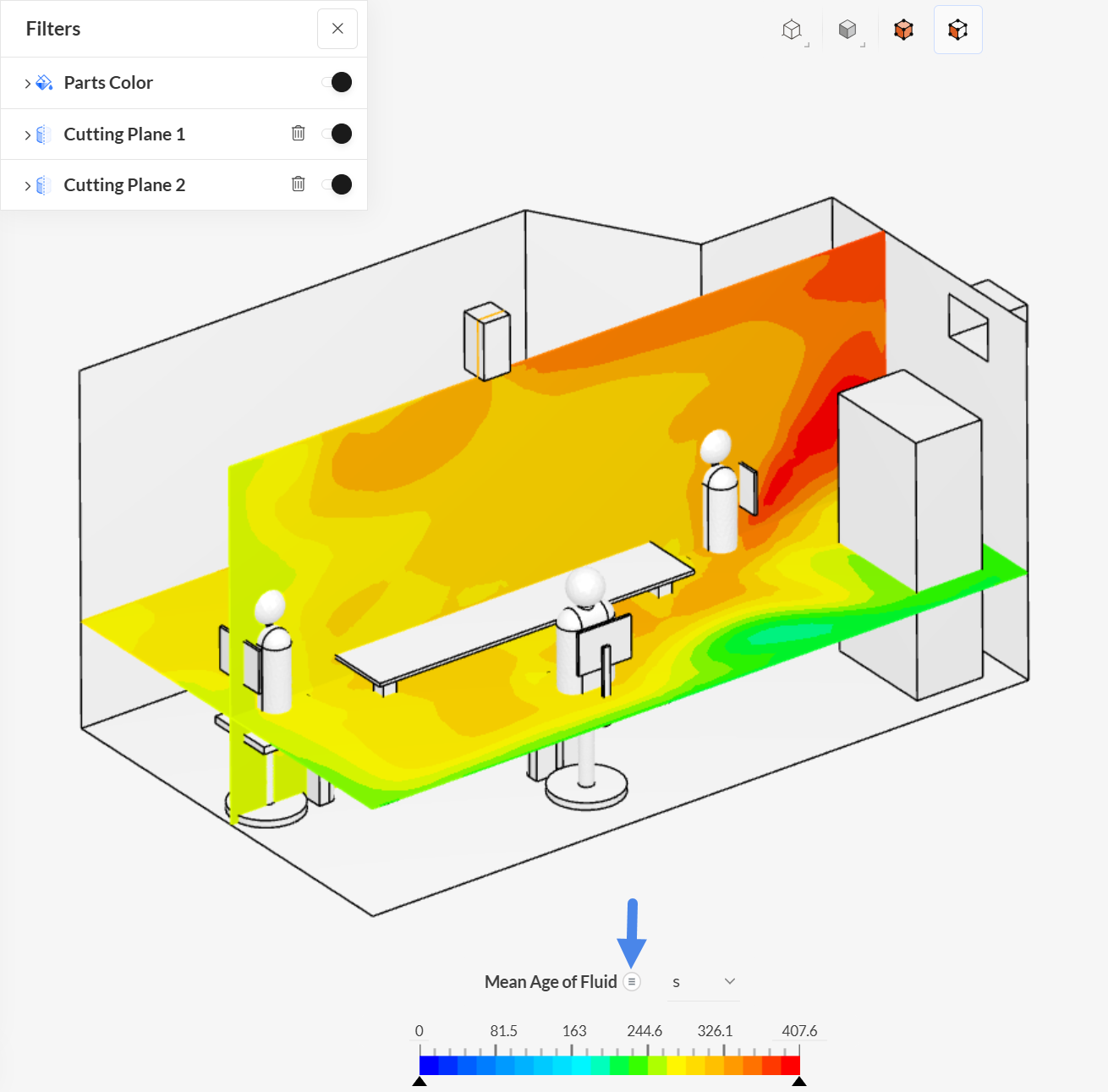
Blue regions show areas with fresh of air and red regions show areas with high age of air. Red areas represent stagnation regions, with poor ventilation.

Analyze and explore your results with the SimScale post-processor. Have a look at our post-processing guide to learn how to use the post-processor.

Congratulations! You finished the tutorial!

Last updated: July 14th, 2026