Advanced Tutorial: Thermal Comfort in a Theater Room
This tutorial analyzes the duct positioning inside of a theater room, aiming to study the effectiveness of the ventilation system and the resulting thermal comfort.
Overview
This tutorial teaches how to:
- Set up and run a thermal comfort simulation
- Assign boundary conditions, material, and other properties to the simulation
- Mesh with the SimScale standard mesher
We are following the typical SimScale workflow:
- Prepare the CAD model for the simulation
- Set up the simulation
- Create the mesh
- Run the simulation and analyze the results
1. Prepare the CAD Model and Select the Analysis Type
First of all, click on the button below. It will copy the tutorial project containing the geometry into your Workbench.
The following image demonstrates what should be visible after importing the tutorial project:

Extract Theater Flow Volume
If you want to perform the flow volume extraction on your own, you can use the ‘Theater – without flow volume extraction’ geometry, we would use the CAD environment. To modify a CAD model, simply select the geometry from the list—the available CAD operations will then appear in the top toolbar. You can either work directly on the original model or create a duplicate and apply your changes to the copy.
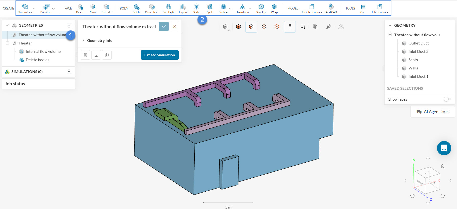
The icon highlighted in Figure 3 will take you to the edit CAD enviroment, where you can perform the flow volume extraction. For more details and instructions, please refer to this article. Additionally, you can have a look at the edited operations performed for the ‘Theater’ geometry and repeat the same.
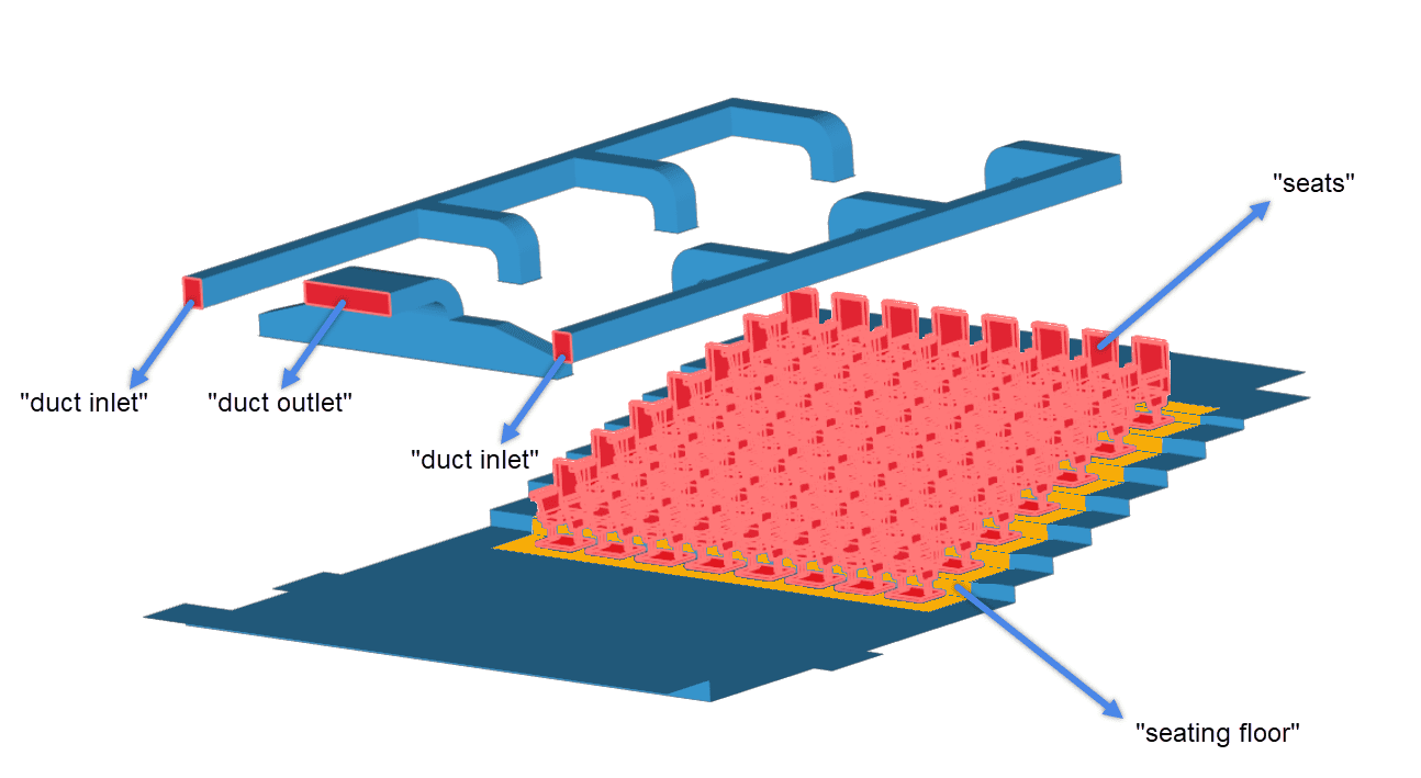
After you extract the flow volume, you can proceed by assigning the following saved selections (notice that in the ‘Theater’ geometry, the saved selections are already created):
- duct outlet
- duct inlet
- seats
- seating floor
For example, to set the saved selection for the duct outlet:
- Click on the outlet of the theater, as you can see below.
- Select the ‘+‘ icon and name it as ‘duct outlet’.
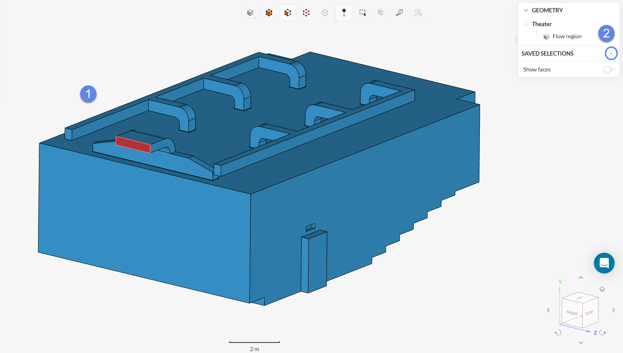
Repeat this for the rest of the sets.
1.1 Create the Simulation
To create a new simulation click on the ‘+’ option next to the ‘Simulations’ tab. Choose ‘Conjugate Heat Transfer’, which is used when temperature changes in the fluid lead to density variations and movement of the fluid due to gravity. Finally, hit the ‘Create Simulation’ button.
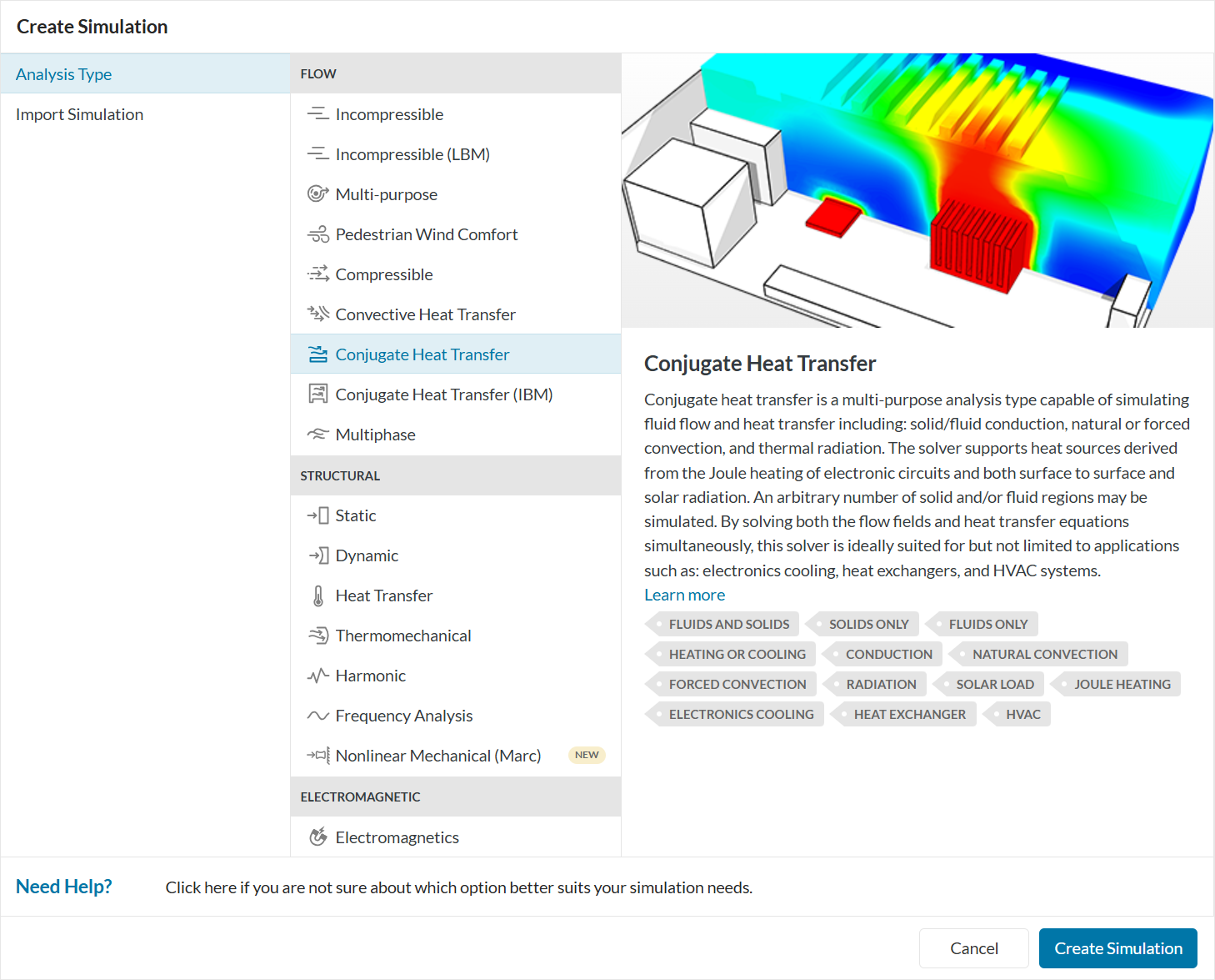
At this point, a new simulation tree will appear. By clicking on the first entry in the simulation tree, you will see the following global settings:
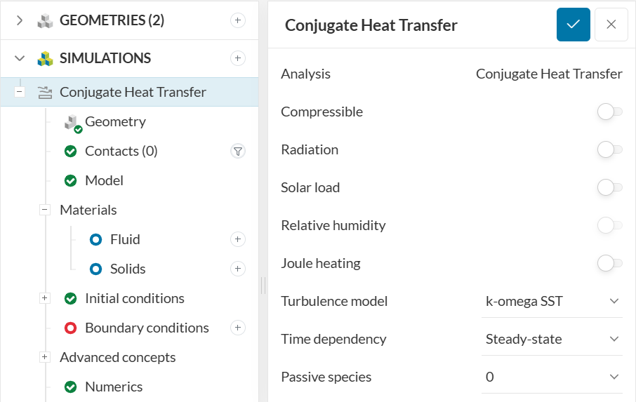
For this tutorial, the ‘k-omega SST‘ turbulence model will be used. This turbulence model blends between the k-omega and k-epsilon models automatically, therefore, it takes advantage of both models.
In reality, all bodies with a temperature greater than absolute zero emit radiation, and in contrast to conduction or convection, this phenomenon requires no medium, so it could also be added. From a practical perspective, radiation is memory-intensive, so it is more often used when the simulation involves high temperature gradients, as it will be more important in these cases. As such, radiation will be off for this tutorial. Learn more about simulating radiation with SimScale here.
2. Assigning the Material and Boundary Conditions
Now we are ready to set up the physics of the simulation. This section includes determining the conditions of the case, from the gravitational load inside the room to the surfaces’ temperature and flow rates.
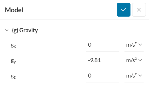
2.1 Define Gravity
Click on ‘Model‘ in the simulation tree to define the gravity force acting on the domain. In this case, gravity is defined in the negative y-direction:
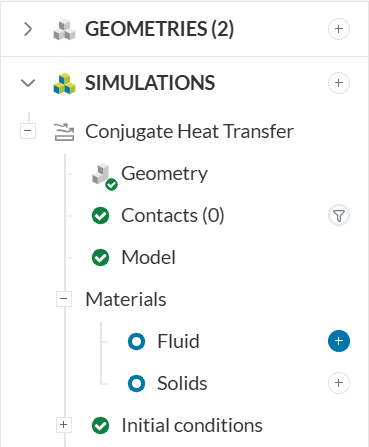
2.2 Define a Material
Click on the ‘+’ icon next to ‘Fluid’ in the Materials tab to start with this assignment:
Assign the standard ‘Air‘ material to the fluid domain by picking it in the material library:
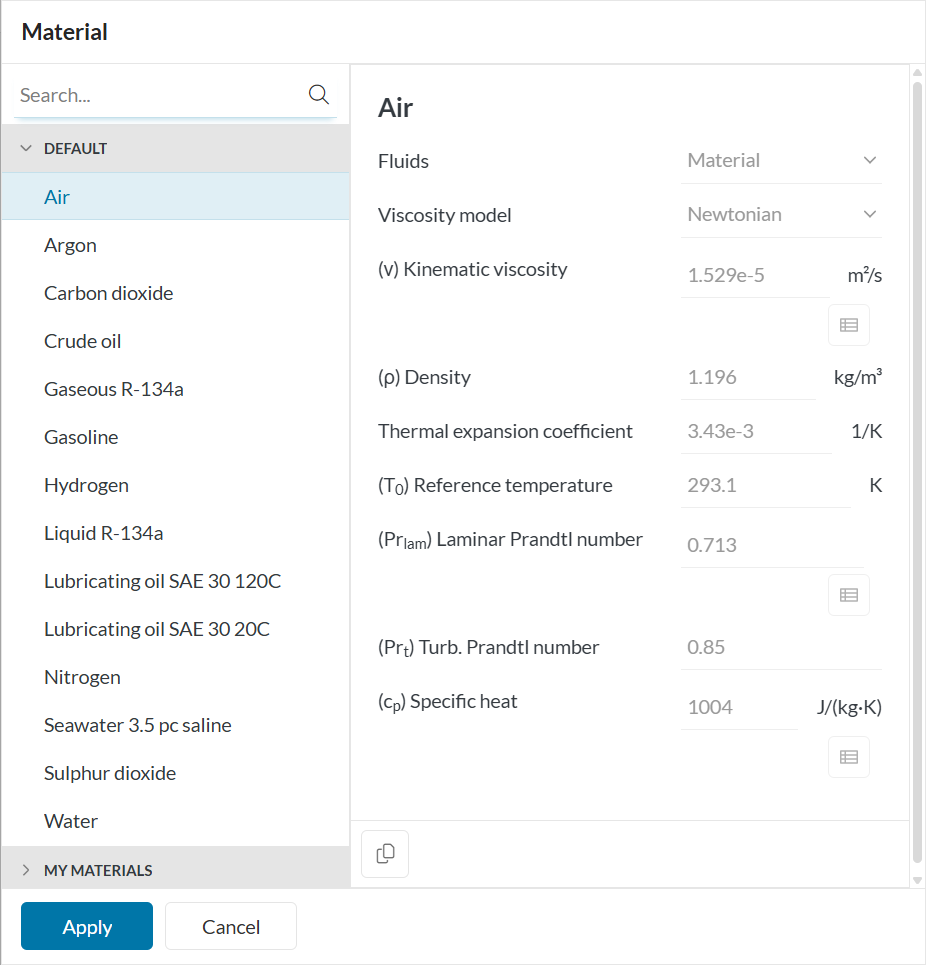
Select ‘Air’ and hit ‘Apply’. Note that you can also just select any material and customize the properties to define whatever material you want to.
Once you have created the new material, you can see the materials data in a new panel:
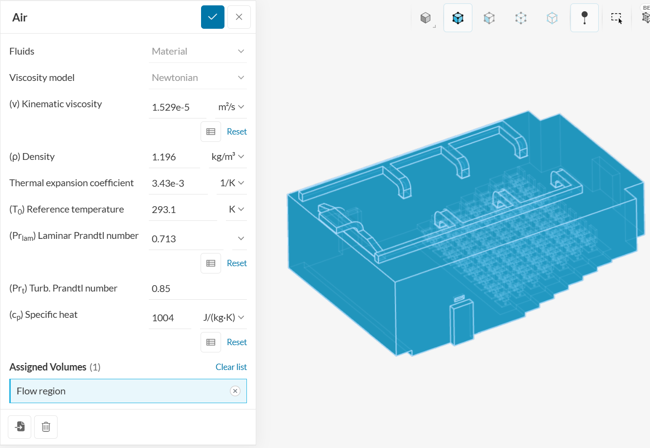
As there is only one volume, the SimScale platform automatically assigns the material to the flow volume. All you need to do here is hit the ‘Check’ button at the top of the panel.
2.3 Initial Conditions
Default values for initial condition parameters are usually enough. Note that those should not affect the result of your simulation. However, if these parameters are estimated reasonably, the solution will converge faster and the overall convergence stability will improve.
2.4 Boundary Conditions
Options for defining boundary conditions for flow simulations
Flow inlet and outlet boundary conditions can be defined in the two following ways:
- Inlet controlled (defining velocity, flow rate, or pressure, on domain inlet).
- Outlet controlled (defining suction velocity, flow rate, or pressure on domain outlet).
Walls can be defined with specific temperature and heat transfer parameters.
While surface heat sources can be defined by ‘fixed temperature‘ or ‘external wall heat fluxes’, adiabatic conditions can be defined by ‘adiabatic’ temperature.
By leaving surfaces unassigned, the default adiabatic no-slip wall condition is applied to them.
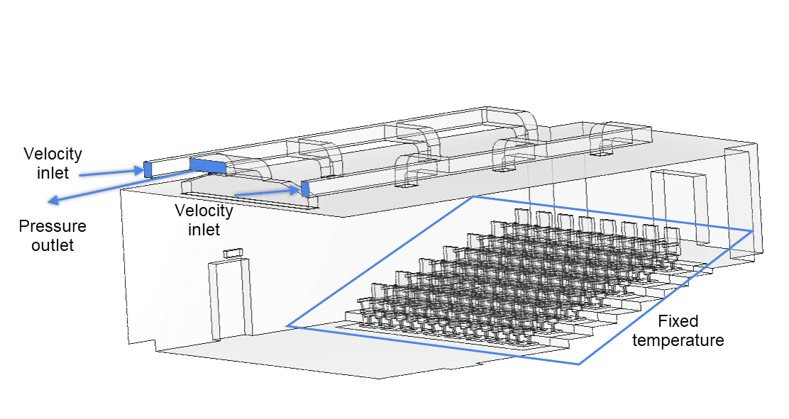
For the boundary condition set up, a velocity inlet and a pressure outlet will be assigned on the air entrances and the exit. The seats will have a fixed temperature value corresponding to the occupants.
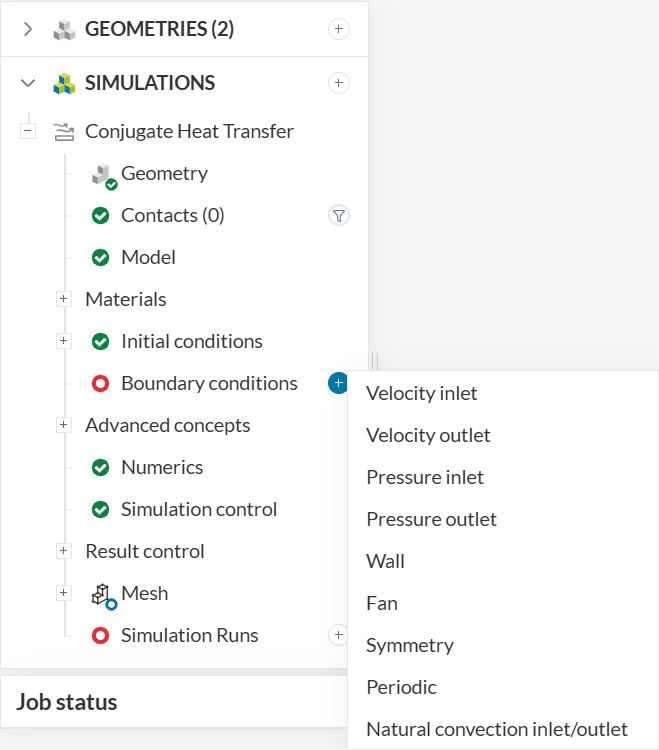
To assign a boundary condition, click on the ‘+‘ icon next to the Boundary conditions. Then choose the desired type on the menu that appears:
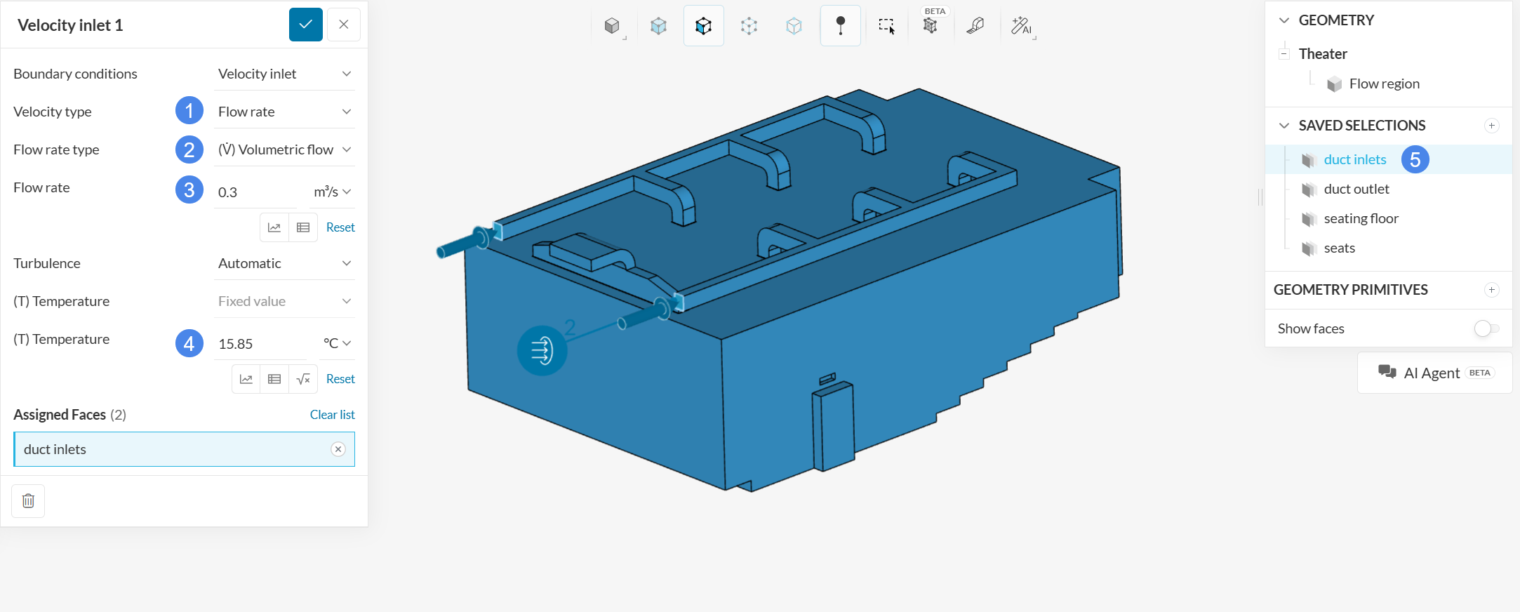
a. Velocity Inlet
As mentioned before, the two duct inlet faces will receive a flow rate input. Add a new velocity inlet condition and follow the steps below:
- Change the Velocity type to ‘Flow rate‘.
- Change the Flow rate type to ‘(V) Volumetric flow’.
- Flow rate: \(V\) = 0.3 \(m^3 \over\ s \).
- Temperature: \(T\) = 15.85 \(°C\).
To assign a boundary condition on a saved selection, proceed to select the desired saved selection from the tree at the right of the page.
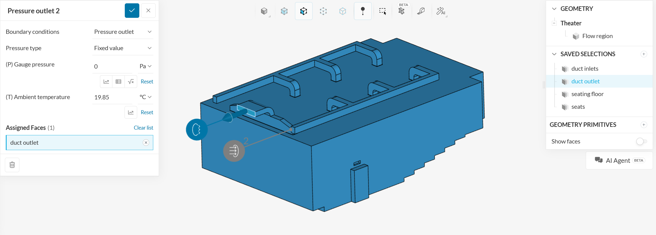
b. Pressure outlet
For the duct outlet face, use a pressure outlet condition with a fixed gauge pressure value: \(P\) = 0 \(Pa\).
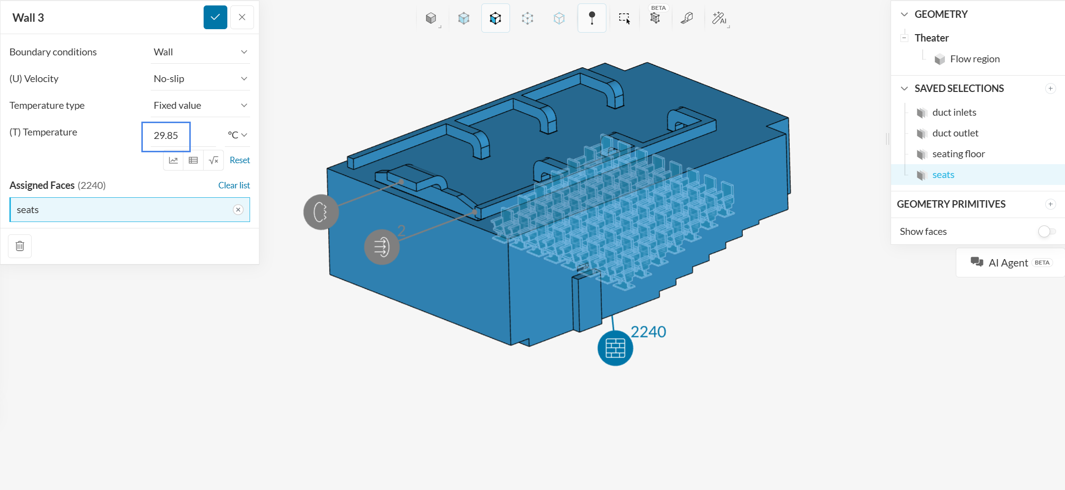
c. ‘No-slip’ walls
For the seats use a no-slip wall condition fixed temperature value: \(T\) = 29.85 \(°C\)
2.5 Set the Numerics & Simulation Control
The default settings for Numerics and Simulation Control are usually suitable. Experienced users can use the manual settings for better convergence. For this thermal comfort tutorial, only change the maximum runtime to 30000 seconds in the simulation control.
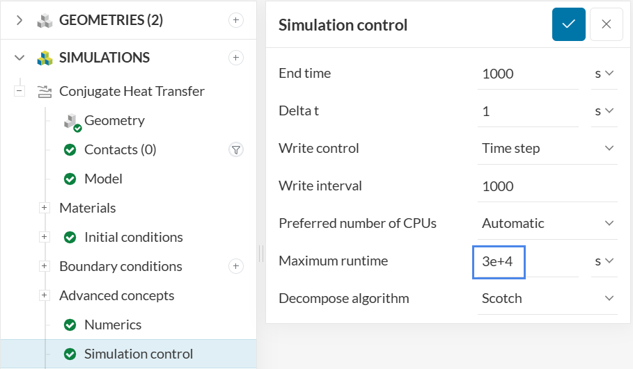
Reminder
The maximum runtime of your simulation is specified in real clock time. When the simulation run surpasses this limit, it will be cancelled.
3. Result Control
Result control items allow us to request the solver to compute special quantities from the simulation, that are not delivered by default. In this case, we will request the Thermal Comfort Parameters fields, as we are interested in these quantities for the evaluation of the results.
For this, create a new Field calculation under Result control, of type ‘Thermal Comfort Parameters’, as shown in the image:
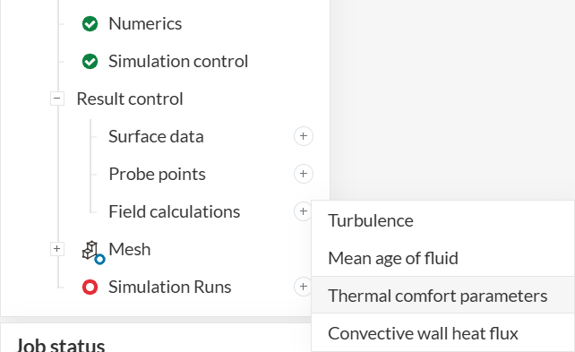
In the setup panel that opens, we can leave the default values and click the blue check-mark button to accept and close.
4. Mesh
Click on ‘Mesh‘ to access the global mesh settings, shown in the following picture. Under Advanced settings, set Small feature suppression to ‘0.005’, which will help to control the cell count by imposing a minimum cell size to the mesh.
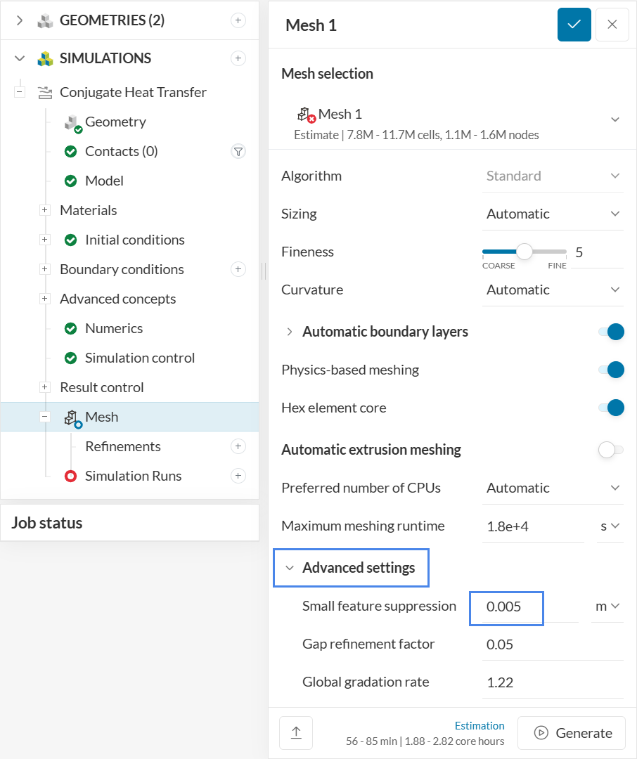
If you are interested to see all configuration options from the standard meshing tool, please take a look at this tutorial.
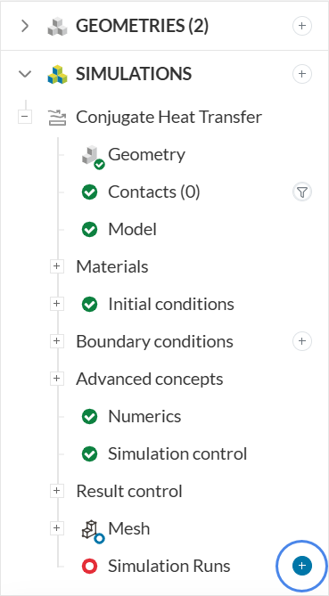
5. Start the Simulation
Create a new run by clicking on the ‘+’ icon next to the ‘Simulation Runs‘:
The mesh will be generated first, and then, while the simulation results are being calculated, you can already have a look at the intermediate results in the post-processor.
6. Post-Processing
For thermal comfort studies, the usual parameters of interest are the PMV (Predicted Mean Vote) and PPD (Predicted Percentage of Dissatisfied). The inputs for those parameters can be found on this page, and the calculated values should be within the following ranges:
- PMV valid range: -3 (cold) to +3 (hot)
- PPD valid range : 5% – 100%
6.1 PMV (Predicted Mean Vote) Parameter
PMV is an index that aims to predict the mean value of votes of a group of occupants on a seven-point thermal sensation scale. Thermal equilibrium is obtained when an occupant’s internal heat production is the same as its heat loss. The heat balance of an individual can be influenced by levels of physical activity, clothing insulation, as well as the parameters of the thermal environment. For example, the thermal sensation is generally perceived as better when occupants have control over indoor temperature (i.e., natural ventilation through an opening or closing windows), as it helps to alleviate high occupant thermal expectations on a mechanical ventilation system.
To comply with the standards, the PMV values should be within these ranges:
- PMV comfort range:
- ASHRAE 55 recommended limit: [-0.5, 0.5]
- ISO 7730:
- Hard limit: [-2, +2]
- New buildings: [-0.5, +0.5]
- Existing buildings: [-0.7, +0.7]
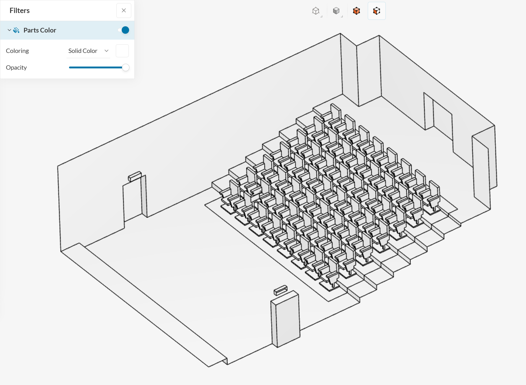
Ideally, from a thermal comfort perspective, the PMV value should be neutral (zero). To analyze the PMV levels around the occupants, let’s start by hiding the ducts and outer walls from the computational domain. The intention is to have a clear view of the inside:

- Initially, delete all other filters and keep Parts Color visible with a solid color, to clean up the viewer
- Enable face selection
- Select the external faces to be removed from the view so that internal faces are visible
- Once the external faces are selected, right-click on the viewer
- Choose the ‘Hide selection’ option
At this point, the interior of the theater will be visible:
A good way to analyze the PMV contours around the seats is with a Cutting plane filter. The following image shows an example:
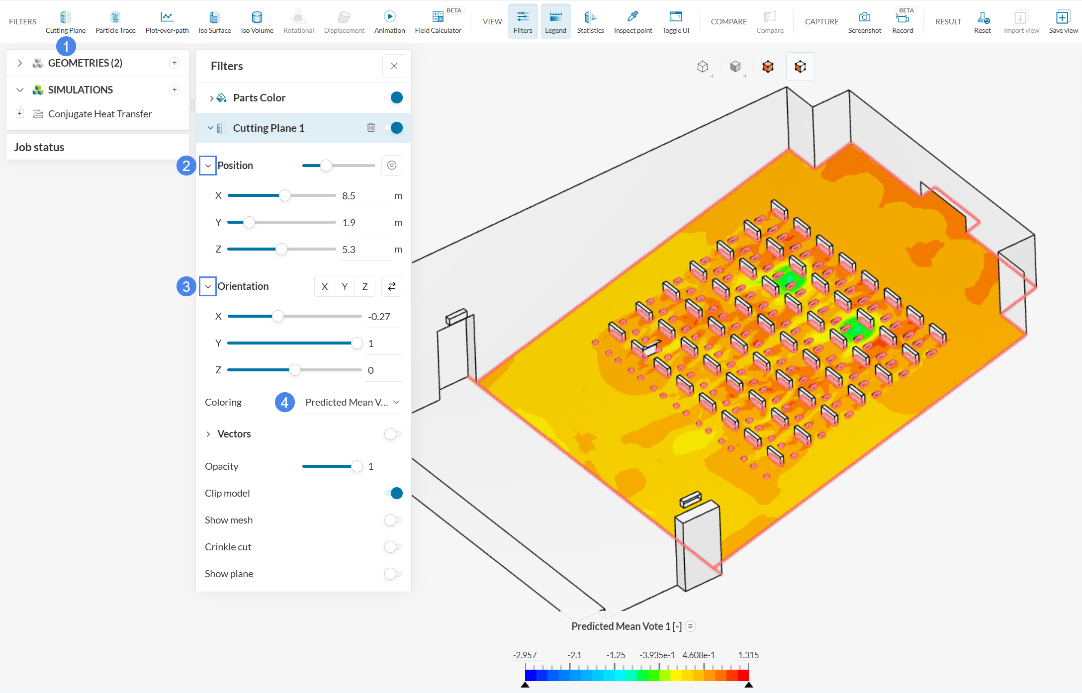
- To create a brand new cutting plane, click on ‘Cutting Plane’ in the filters ribbon
- Expand the Position tab and set X, Y, and Z to ‘8.5’, ‘1.9’, and ‘5.3’ meters, respectively
- Since the seats go up at an angle, you can expand the Orientation tab and adjust the normal directions to ‘-0.27’ in X, ‘1’ in Y, and ‘0’ in Z
- Finally, adjust the Coloring to ‘Predicted Mean Vote’.
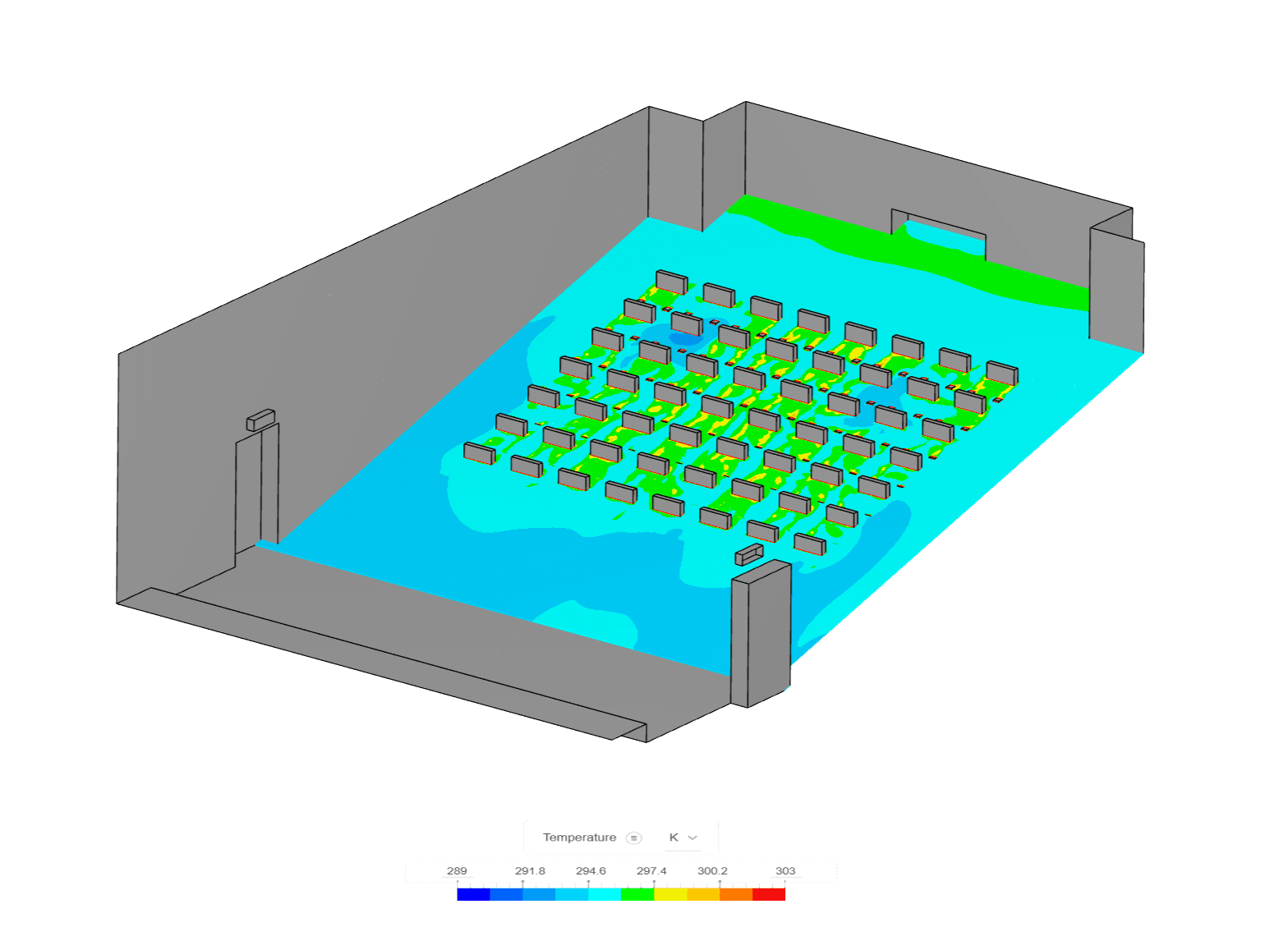
Now the PMV value around the seats is visible, with some regions extrapolating the 0.5 PMV threshold, as well as two small regions with PMV less than -0.5.
6.2 PPD (Predicted Percentage of Dissatisfied) Parameter
PPD essentially gives the percentage of people predicted to experience local discomfort. The main factors causing local discomfort are unwanted cooling or heating of an occupant’s body. Common contributing factors are draft, abnormally high vertical temperature differences between the ankles and head, or floor temperature.
According to the PPD ASHARE 55, the recommended comfort range is: [0%, 20%]. By using the same cutting plane that was created previously, adjust the Coloring to ‘Predicted Percentage of Dissatisfied’:
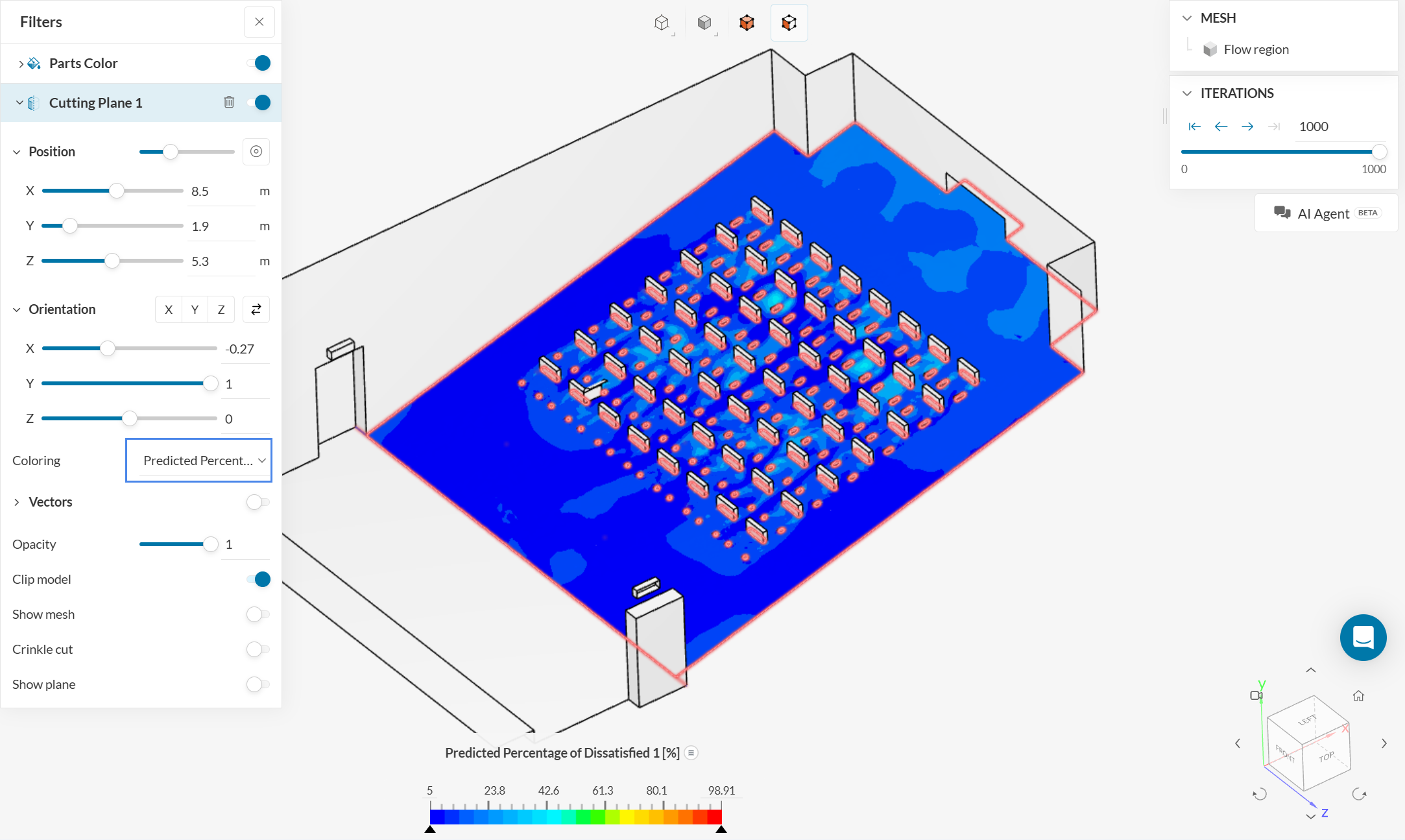
Both the PMV and PPD results show no compliance with the standards for the thermal comfort of this theater, so new measures regarding the ducting should be taken into account to improve them. To learn more about these parameters, visit this blog post: What Is PMV? What Is PPD? The Basics of Thermal Comfort.
Have a look at our post-processing guide to learn how to use the post-processor.
Congratulations! You finished the tutorial!
Note
If you have questions or suggestions, please reach out either via the forum or contact us directly.
Last updated: April 6th, 2026
Did this article solve your issue?
How can we do better?
We appreciate and value your feedback.


