Documentation
This validation case belongs to solid mechanics. The aim of this test case is to validate the following parameters:
The simulation results of SimScale were compared to the results from [SDLS109]\(^1\).
The geometry used for the frequency analysis is as follows:
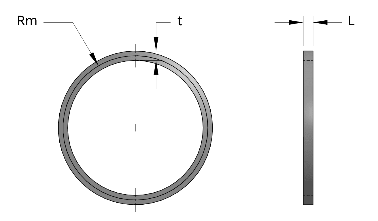
The ring has a length \(L\) of 0.05 \(m\), a thickness \(t\) of 0.048 \(m\), and a medium radius \(Rm\) of 0.369 \(m\).
Tool Type: Code_Aster
Analysis Type: Frequency Analysis
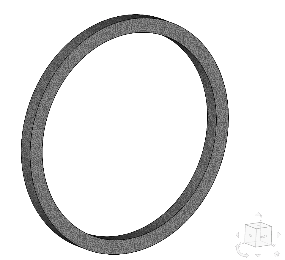
Mesh and Element Types:
First and second order meshes were computed using the SimScale standard mesh algorithm:
| Case | Mesh Type | Number of Nodes | Element Type |
|---|---|---|---|
| A | 1st Order Tetrahedral | 24755 | Standard |
| B | 1st Order Tetrahedral | 24755 | Standard |
| C | 1st Order Tetrahedral | 24755 | Standard |
| D | 2nd Order Tetrahedral | 172165 | Standard |
| E | 2nd Order Tetrahedral | 172165 | Standard |
| F | 2nd Order Tetrahedral | 172165 | Standard |
A mesh independence study was also performed for the second order meshes and IRAM – Sorensen algorithm to ensure the optimal fineness parameter level.
| Mesh # | Mesh Type | Number of Nodes | Mesh Fineness |
|---|---|---|---|
| 1 | 2nd Order Tetrahedral | 677 | 2 |
| 2 | 2nd Order Tetrahedral | 1443 | 4 |
| 3 | 2nd Order Tetrahedral | 3557 | 6 |
| 4 | 2nd Order Tetrahedral | 14004 | 8 |
Material:
Boundary Conditions:
Computing Algorithm:
The following available computing algorithms were compared in the different cases:
| Case | Natural Frequencies Computing Algorithm |
|---|---|
| A | IRAM – Sorensen |
| B | Lanczos |
| C | Bathe – Wilson |
| D | IRAM – Sorensen |
| E | Lanczos |
| F | Bathe – Wilson |
The main characteristics of each algorithm are summarized below [U4.52.02]\(^2\):
A fourth algorithm is also available in SimScale, called QZ. This algorithm suffers from high memory consumption, which limits its application to cases with less than 1000 degrees of freedom. Therefore, it is not suitable for the current validation case.
Note
Complex matrices appear in the frequency analysis of materials with frequency damping. As this model is not available in SimScale, the difference between the algorithms comes down to robustness and speed.
The reference solution is of numerical type, as developed in [SDLS109]\(^1\). The solution is presented in terms of all the natural frequencies and their corresponding shapes in the frequency range [200, 800] \(Hz\). This solution was achieved by a convergence analysis using hexahedral elements, and as reported in the reference, a precision of 5% of the computed frequencies is estimated.
The consulted reference solution is:
| Mode | Natural Frequency \([Hz]\) |
|---|---|
| Ovalization | 210.55 |
| 210.55 | |
| Trifoliate | 587.92 |
| 587.92 | |
| Out of Plane | 205.89 |
| 205.89 | |
| 588.88 | |
| 588.88 |
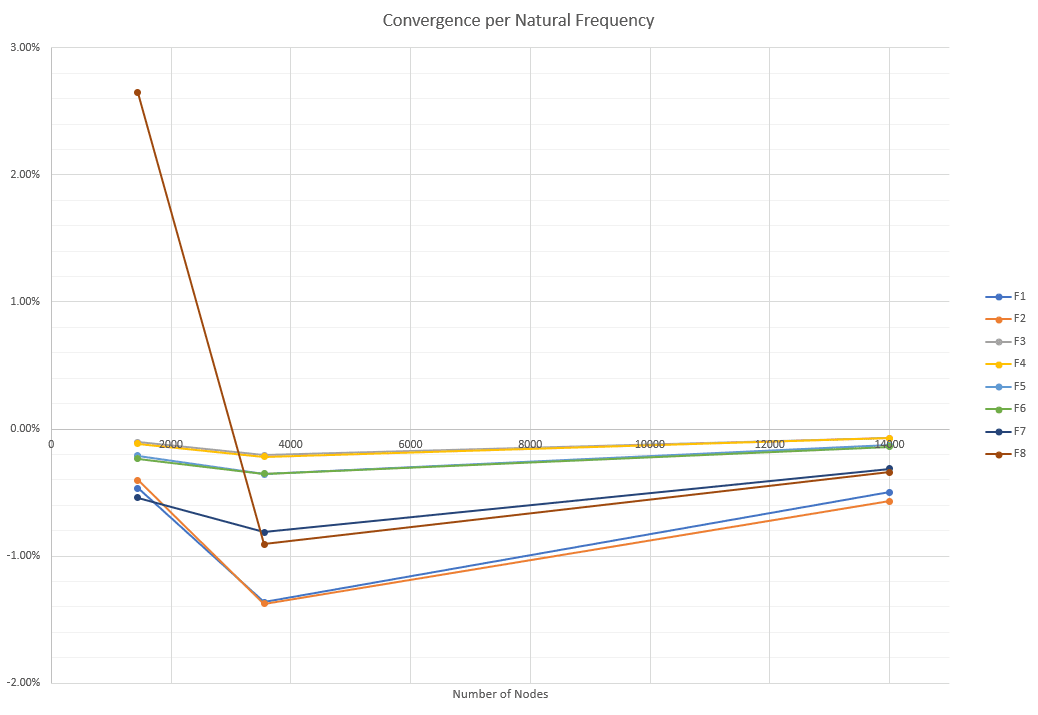
Below can be found the results of the mesh independence study. For each natural frequency (F1 through F8), the variation of the result (in percent) with respect to the previous solution is plotted against the number of nodes in the mesh. At the final, finer mesh, the solution precision is 0.6% or lower.
Comparison of computed natural frequencies with the reference solution for each case can be seen below:
| Mode | Reference Solution | SimScale Solution | Error |
|---|---|---|---|
| Ovalization | 210.55 | 213.332 | 1.32 % |
| | 210.55 | 213.966 | 1.62 % |
| Trifoliate | 587.92 | 596.343 | 1.43 % |
| | 587.92 | 596.698 | 1.49 % |
| Out of Plane | 205.89 | 210.017 | 2.00 % |
| | 205.89 | 210.244 | 2.11 % |
| | 588.88 | 599.512 | 1.81 % |
| | 588.88 | 599.521 | 1.81 % |
| Mode | Reference Solution | SimScale Solution | Error |
|---|---|---|---|
| Ovalization | 210.55 | 215.181 | 2.20 % |
| | 210.55 | 216.09 | 2.63 % |
| Trifoliate | 587.92 | 601.83 | 2.37 % |
| | 587.92 | 602.316 | 2.45 % |
| Out of Plane | 205.89 | 212.822 | 3.37 % |
| | 205.89 | 213.098 | 3.50 % |
| | 588.88 | 606.685 | 3.02 % |
| | 588.88 | 606.794 | 3.04 % |
| Mode | Reference Solution | SimScale Solution | Error |
|---|---|---|---|
| Ovalization | 210.55 | 209.998 | -0.26 % |
| | 210.55 | 209.998 | -0.26 % |
| Trifoliate | 587.92 | 586.293 | -0.28 % |
| | 587.92 | 586.293 | -0.28 % |
| Out of Plane | 205.89 | 205.143 | -0.36 % |
| | 205.89 | 205.144 | -0.36 % |
| | 588.88 | 586.975 | -0.32 % |
| | 588.88 | 586.975 | -0.32 % |
Results are mesh dependent instead of algorithm dependent because all algorithms produce similar results. The difference between algorithms can be seen when looking at the running times. Cases using IRAM – Sorensen and Lanczos algorithm are much faster than Bathe – Wilson. The recommendation is then to stay with the default algorithm (IRAM – Sorensen), because of its known robustness.
| Algorithm | Runtime 1st Order Mesh | Runtime 2nd Order Mesh |
|---|---|---|
| IRAM – Sorensen | 2 min | 13 min |
| Lanczos | 2 min | 13 min |
| Bathe – Wilson | 9 min | 139 min |
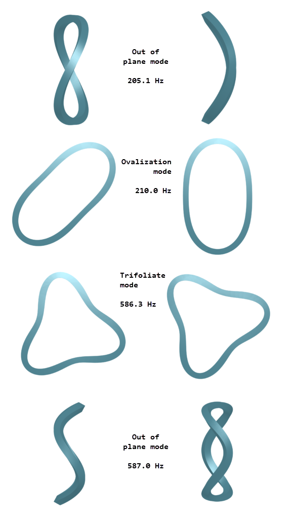
Following are the referenced natural mode shapes as seen on the online post-processor:
References
Note
If you still encounter problems validating you simulation, then please post the issue on our forum or contact us.
Last updated: June 30th, 2020
We appreciate and value your feedback.
Sign up for SimScale
and start simulating now