Documentation
In this tutorial, a compressible aerodynamic simulation of a golf ball is performed.
This tutorial teaches how to:
We are following the typical SimScale workflow:
Attention!
This tutorial performs simulation with the Compressible analysis type which is only accessible to users with a Professional plan and those who are already on the Community plan. New Community users or those recently downgraded to the Community plan will not longer be able to perform this tutorial. See our pricing page to request additional features.
First of all, click the button below. It will copy the tutorial project containing the geometry into your own Workbench.
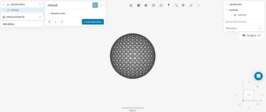
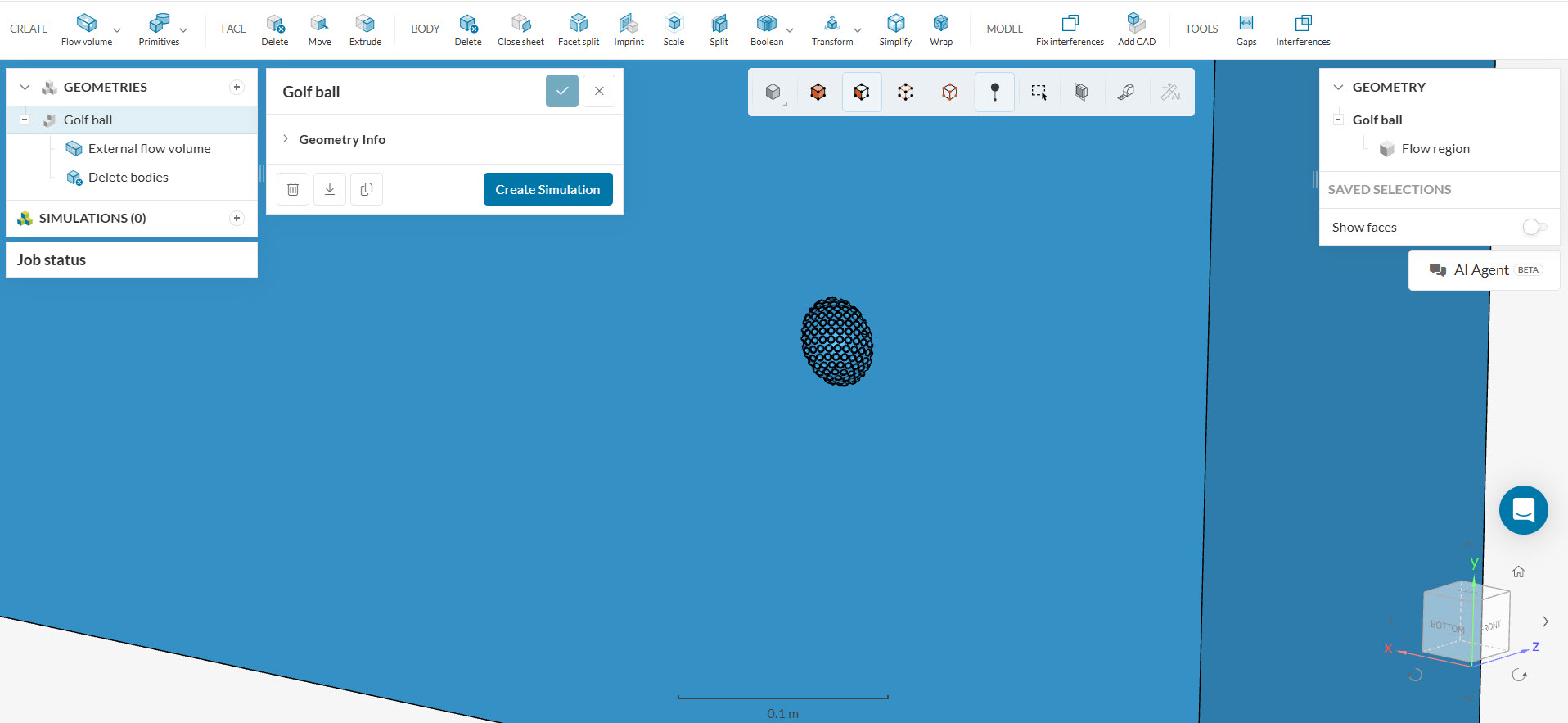
The following picture demonstrates what should be visible after importing the tutorial project.
The first step for this simulation is the creation of a flow region volume. This will be the domain used for the external CFD analysis. To perform the necessary operations, simply select the geometry from the list—the available CAD operations will then appear in the top toolbar. You can either work directly on the original model or create a duplicate and apply your changes to the copy.
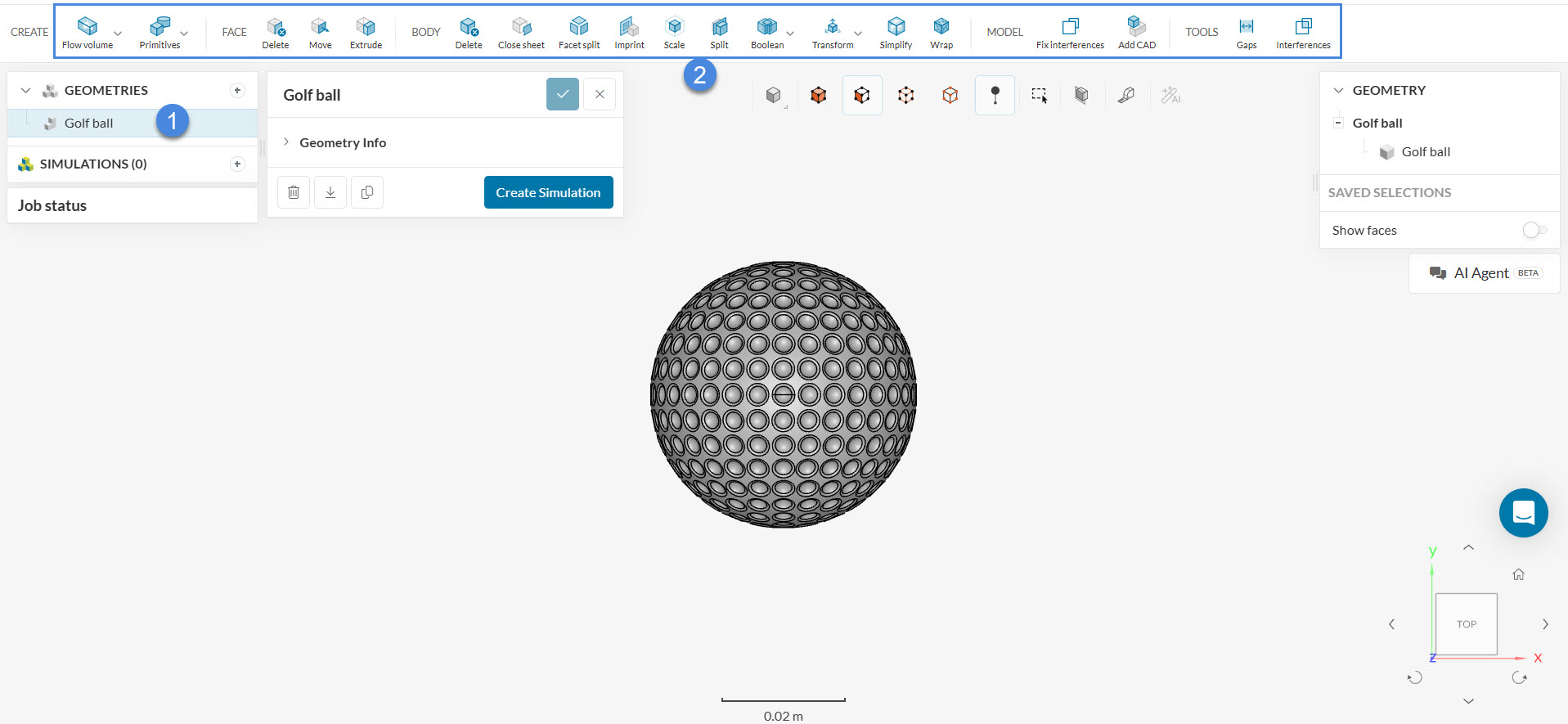
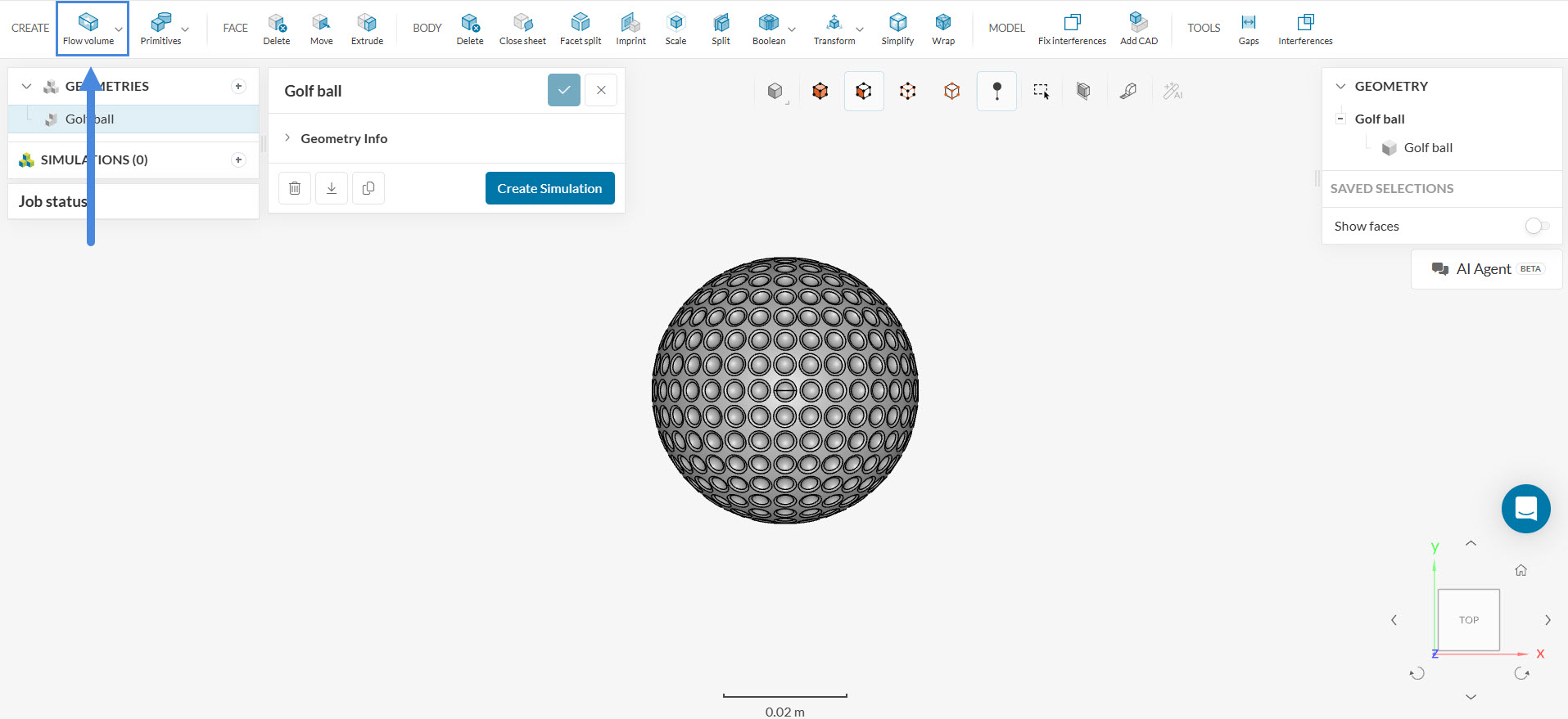
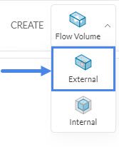
Select ‘Create – Flow volume’, from the top bar:
The ‘External’ option that is listed on the drop-down menu is used to create the flow domain around the model:
Then, fill in the dimensions of the domain as shown below. Here, L represents the diameter of the golf ball:

In more detail, the dimensions of the domain are as follows. Notice that only half of the domain is included, to leverage the symmetry of the model and save computational resources:
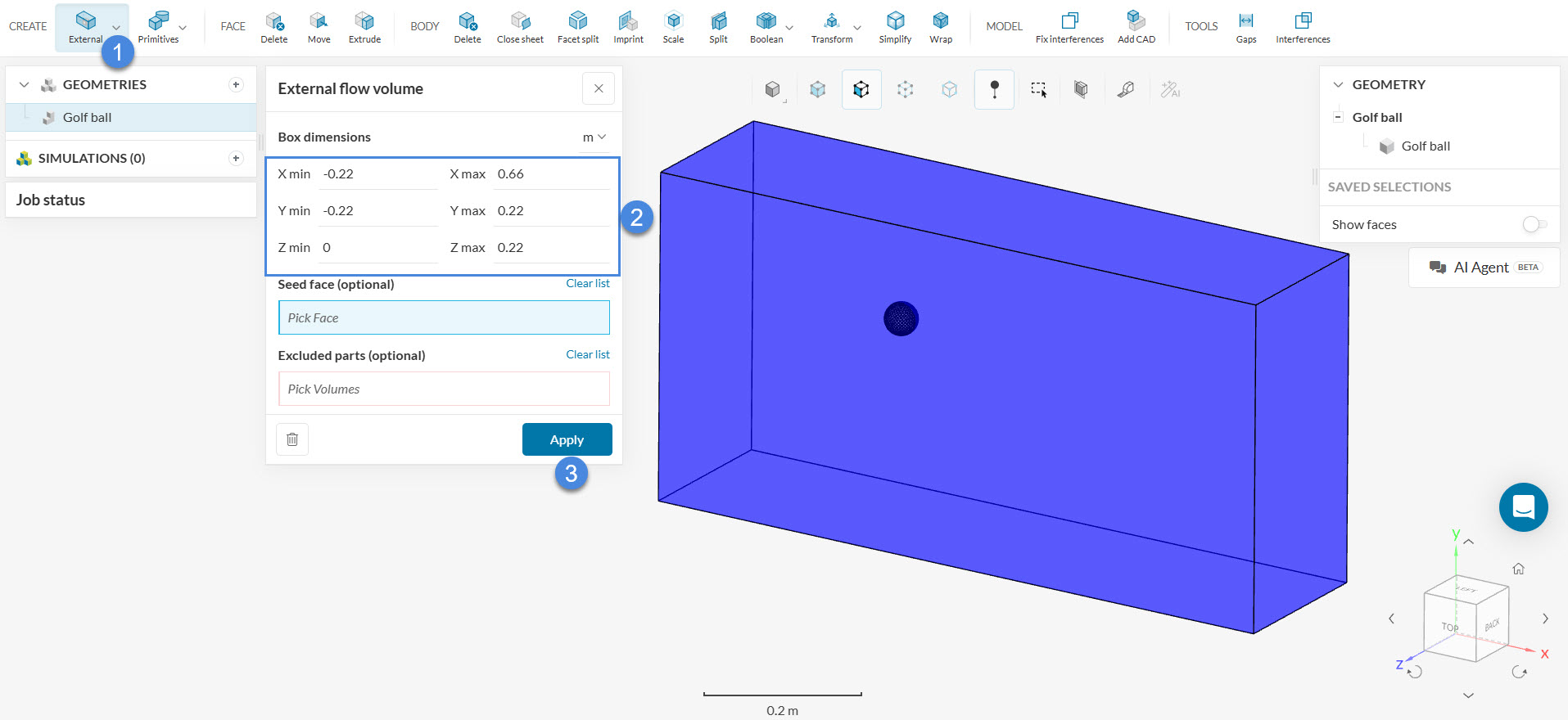
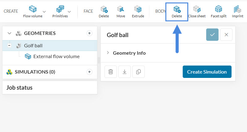
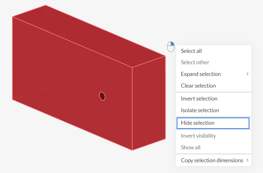
After you are done, click ‘Apply‘. Then select the ‘Delete’ feature below the Body section, to remove the solid part representing the ball:
Select the solid body from the scene tree on the right and click ‘Apply’:
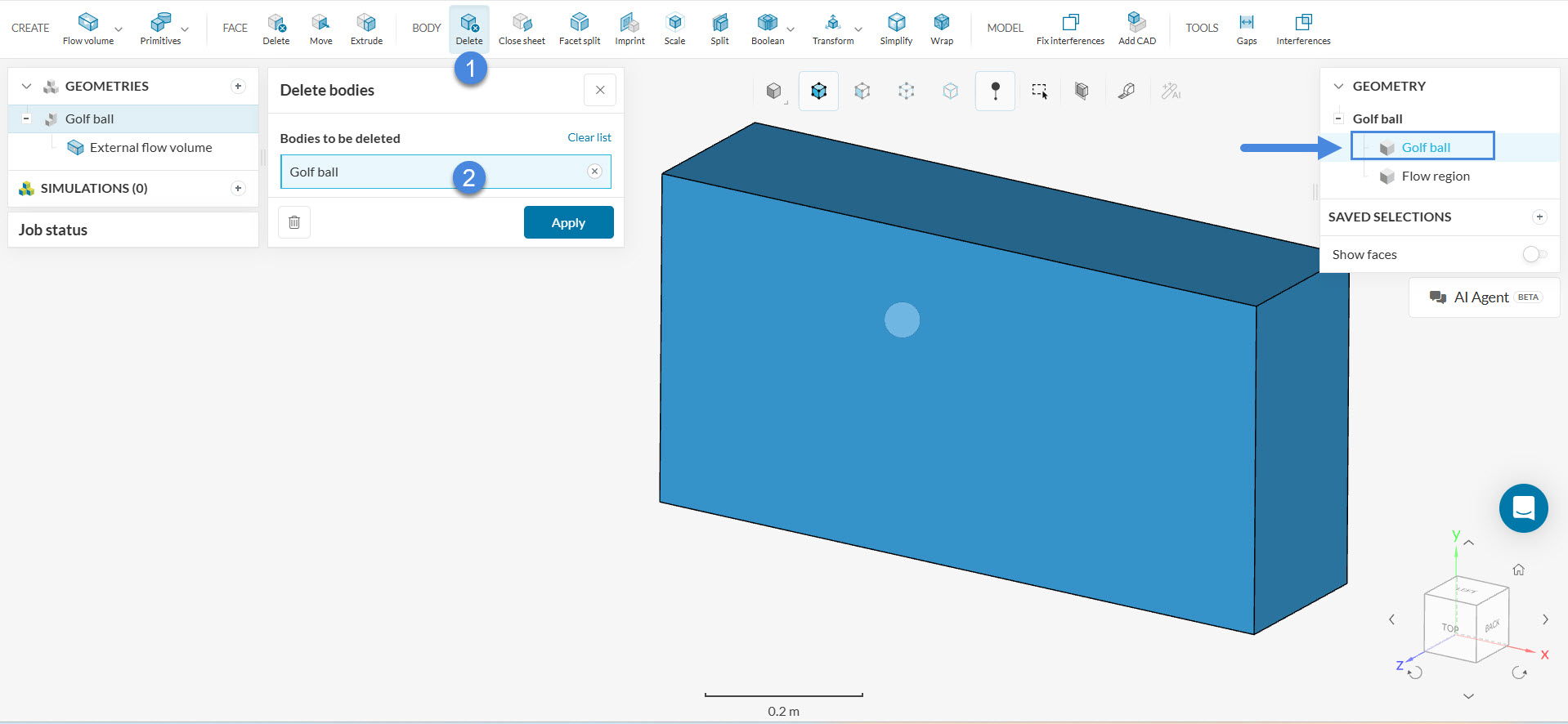
When the operation is finished and the ball is removed, the geometry will be ready. All the changes made should be applied to the original geometry listed, unless a duplicate of it is being worked on.
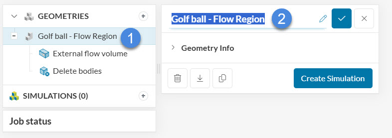
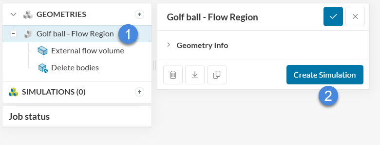
When all the modifications are made, the changes will appear under the geometry in the Geometries list.
Then, rename the new version as ‘Golf ball – Flow Region’:
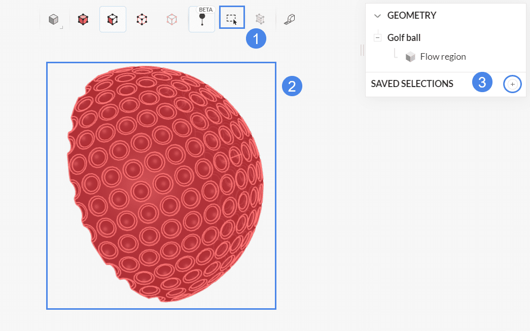
Create a Saved Selection for the golf ball surface:
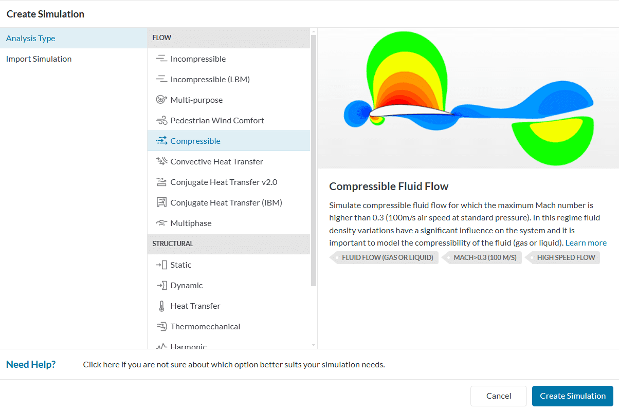
After you finish with the creation of saved selections, proceed to click the ‘Create simulation‘ option to get started.
Select the ‘Compressible‘ analysis, which is used for cases where the Mach number in any point of the domain reaches a value bigger than 0.3. This golf ball simulation will be using a high velocity, so the compressible analysis is the best fitting.
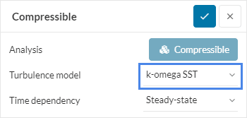
Switch the Turbulence model to ‘k-omega SST‘ in the panel that appears:
Now we will set up the physics for the simulation.
In this simulation, we want to analyze the airflow around a solid body. Therefore we need to assign properties to the fluid region. Click on the ‘+’ icon next to the Materials option of the simulation tree on the left panel, then choose ‘Air‘ in Material pop up, and finally Apply:
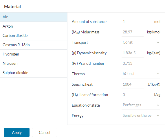
The flow region that was created in the CAD editing at the beginning of the tutorial is automatically selected for the material, because it is the only one present.
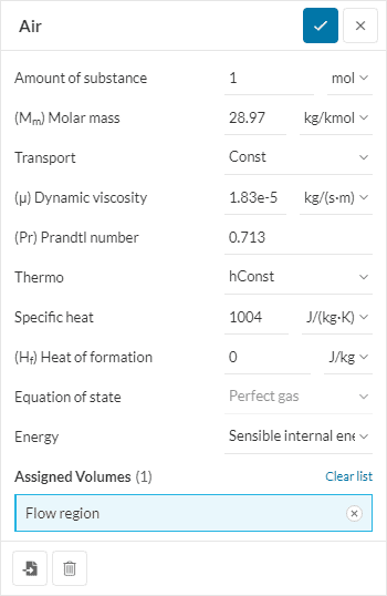
Just confirm the selection by hitting the check button at the top of the panel. You can also create a custom fluid by changing the parameters and giving it a proper name.
In order to assign Boundary Conditions on the model, click on the ‘+’ icon next to the Boundary Conditions, and select the types described in this section.

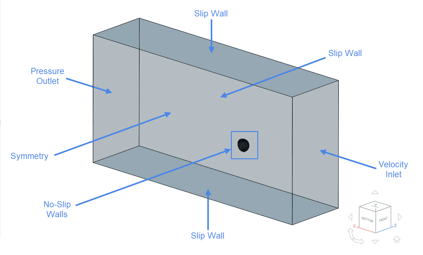
The following picture shows an overview of the boundary conditions used in this simulation:
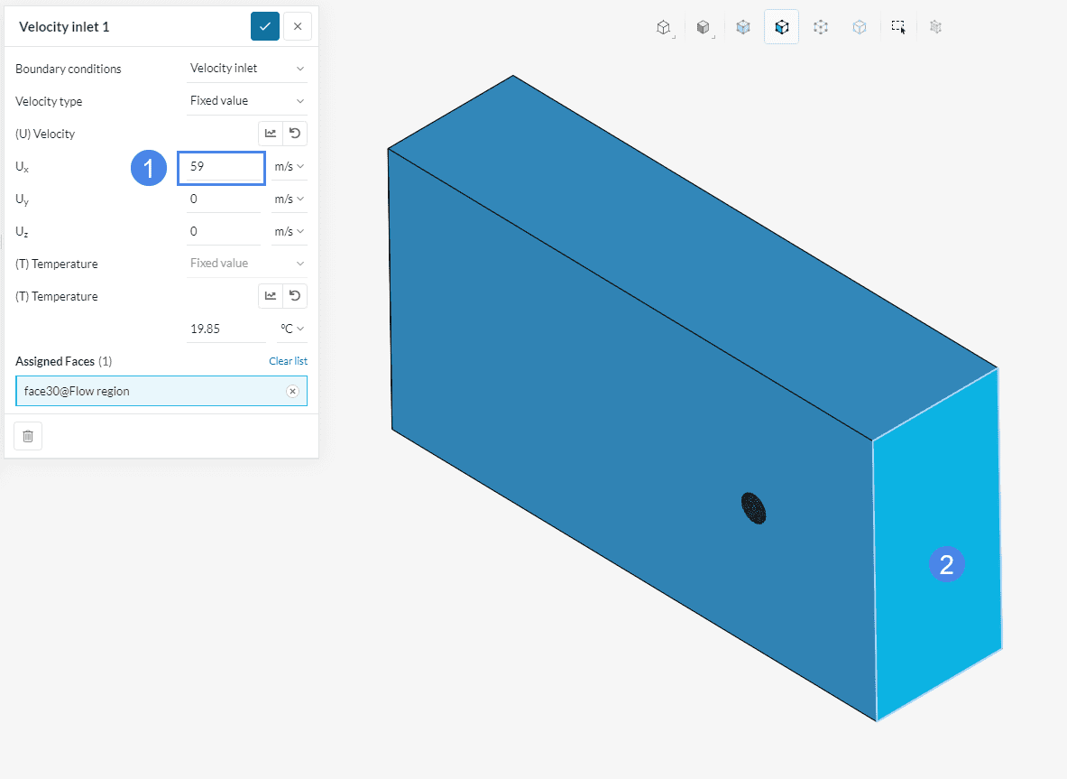
a. Velocity Inlet
Assign a ‘Velocity Inlet‘ of 59 \(m/s\). This value is close to the Ball Speed that an average male golf player achieves[1].
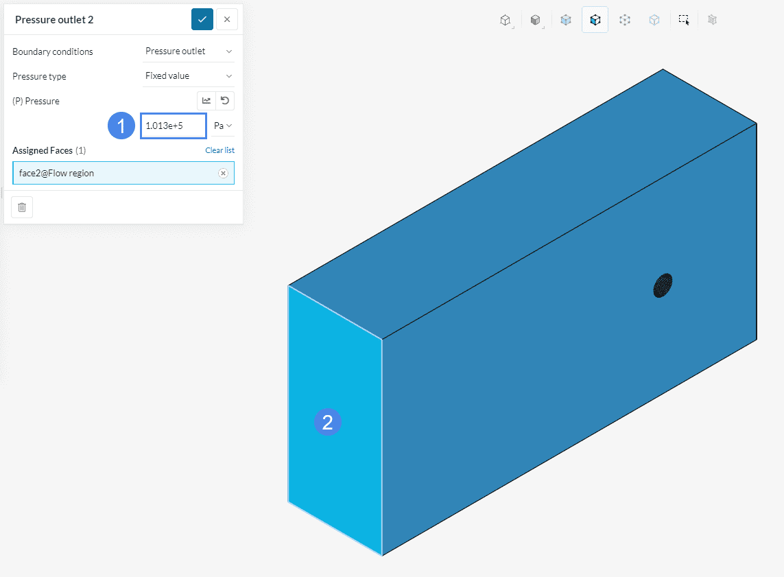
b. Pressure Outlet
Assign a ‘Pressure Outlet‘ condition of 101 325 (Pa) at the highlighted face below:
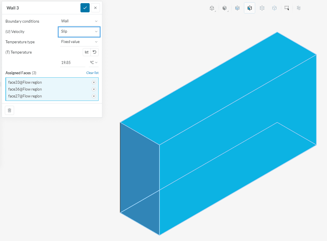
c. Slip Walls
Add a Slip Wall boundary condition on the top, bottom, and right faces of the domain. Leave the symmetry plane unassigned.
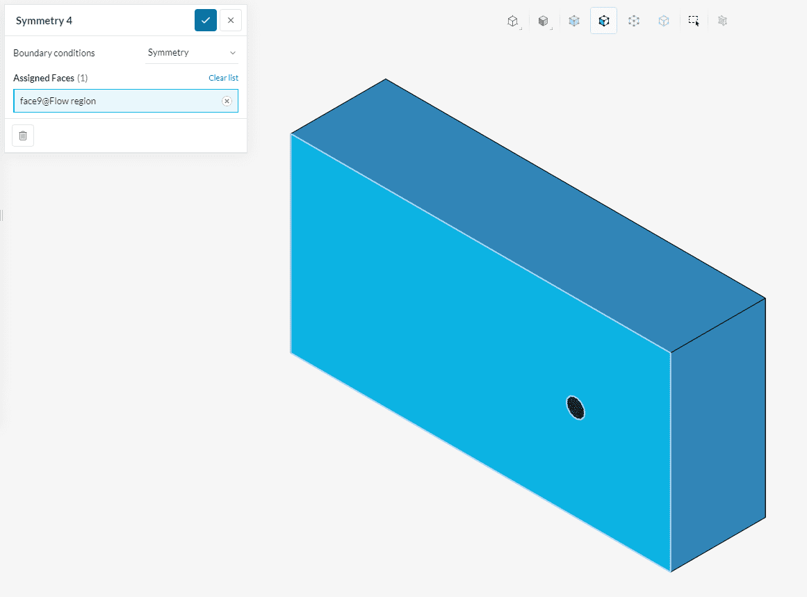
d. Symmetry
Assign a Symmetry condition on the symmetry cut plane. If you want to learn more about this boundary condition, click here.
e. Rotating Walls
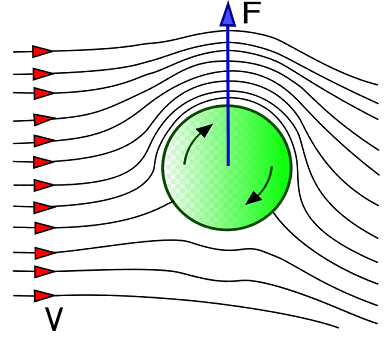
Did you know?
The golf ball rotates like the in following figure, thus the negative z direction is chosen for the rotation axis.
We will define the condition according to the spin rate of an average male golf player. Create a new ‘wall’ boundary condition:
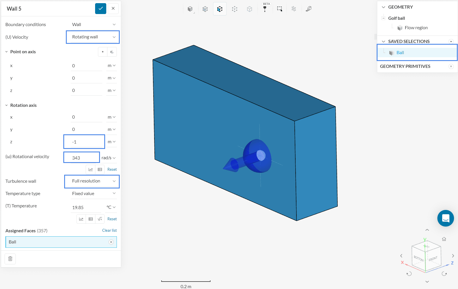
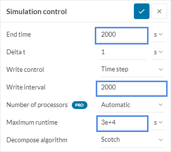
Fill the simulation control panel parameters like below:
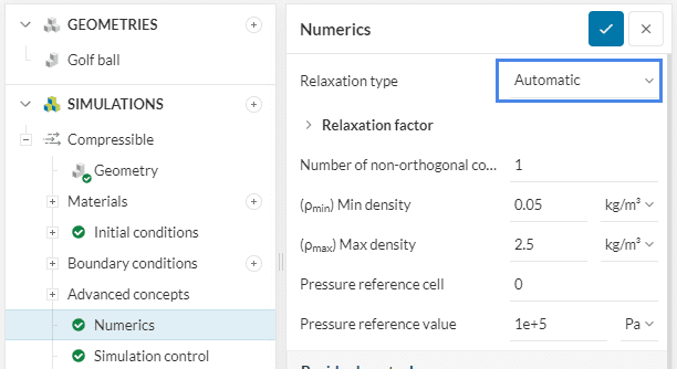
Under Numerics, please make sure that the Relaxation type is set to ‘Automatic’:
Access the global mesh settings by clicking on ‘Mesh’ in the simulation tree:
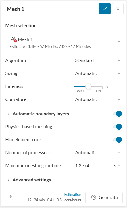
Choose the ‘Standard‘ algorithm, and keep the default settings.
This project needs some mesh refinements in the region around the golf ball. If you want to learn more about using the Standard meshing tool, and using refinements, click on this.
a. Create Geometry Primitives
Prior to adding refinements, you must create some Geometry Primitives.

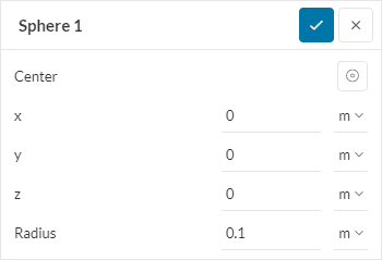
Create a second Sphere primitive with a smaller radius (‘0.05’ \(m\)):

b. Assign Volume Custom Sizing to the Spheres
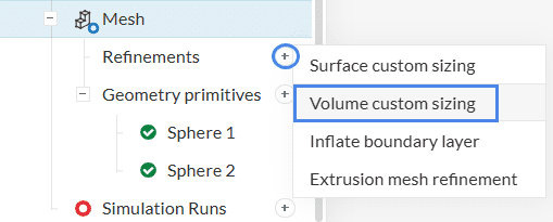
In order to add a volume custom sizing, click on ‘+’ icon next to Refinements under Mesh:
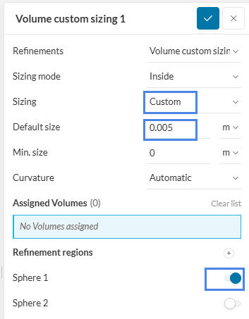
Add a volume custom sizing to the first sphere:
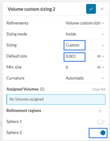
And a second, finer volume custom sizing to the smaller sphere, to create a denser mesh:
Watch out!
Do not click on the ‘Generate’ button after you are done with the mesh settings. Instead of generating the mesh at this point, it will be automatically created after you start the simulation run later on.
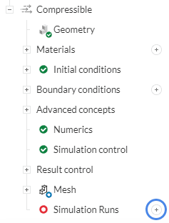
After all the settings are completed, proceed to clicking the ‘+’ icon next to the Simulation Runs, in order to get started with the computation. Initially, your mesh will be generated, and then the platform will go on with the run.
While the computation is running, you can have a look at the intermediate results in the post-processor.
Did you know?
Your results are being updated in real time! That means that you can already look into the intermediate results while the solver computes the final solution.
When the simulation is completed, you can check the convergence of the simulation. You can access it under the completed run:
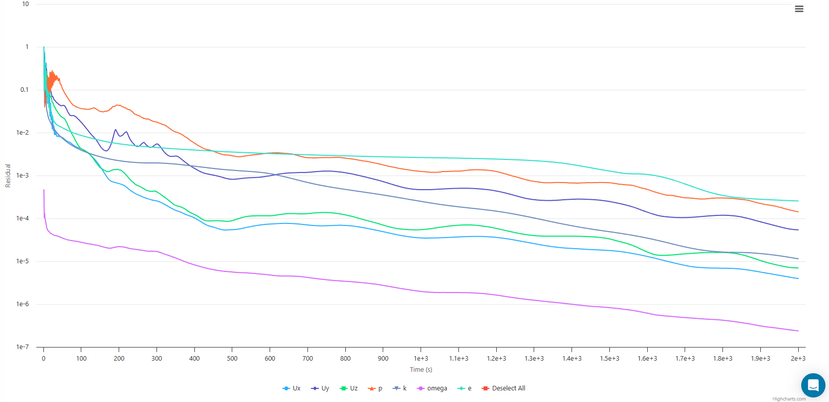
The convergence plot indicates whether the solution is reliable, or whether some changes should be made in the settings. For example, making the mesh finer, or increasing the simulation time. In the following picture you can see how the convergence of the residuals of your simulations will appear in the plot:
In order to view the results of your golf ball simulation, click on the ‘Solution Fields’ tab under your finished run. This will redirect you to the online graphical post-processor.
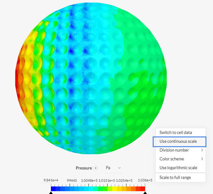
You can use several post-processing filters to further analyze the results. For instance, if you wish to see the pressure distribution on your golf ball :
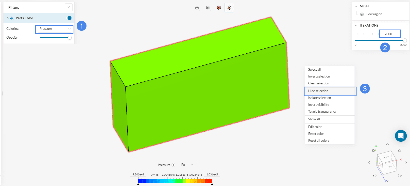
Make sure to right-click on the color scale at the bottom of the screen and select the ‘Use continuous scale option’, for smoother transition between color contours:
This is how the results will appear afterwards, if you include the symmetry plane too:
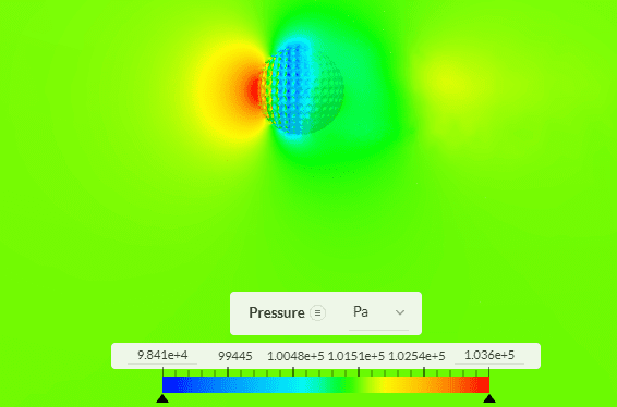
It is seen that at the front of the ball, an area of high pressure is created, and a low-pressure region is observed at the back. As the velocity is decelerating when reaching the back of the ball, there is flow separating, resulting in this low-pressure area.
Finally, for streamline visualization, select ‘Particle Trace’ from the top bar:

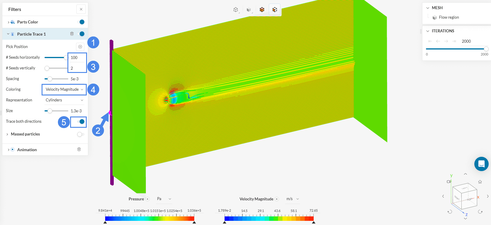
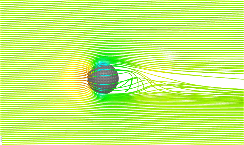
With these settings, this is how the streamlines will finally appear:
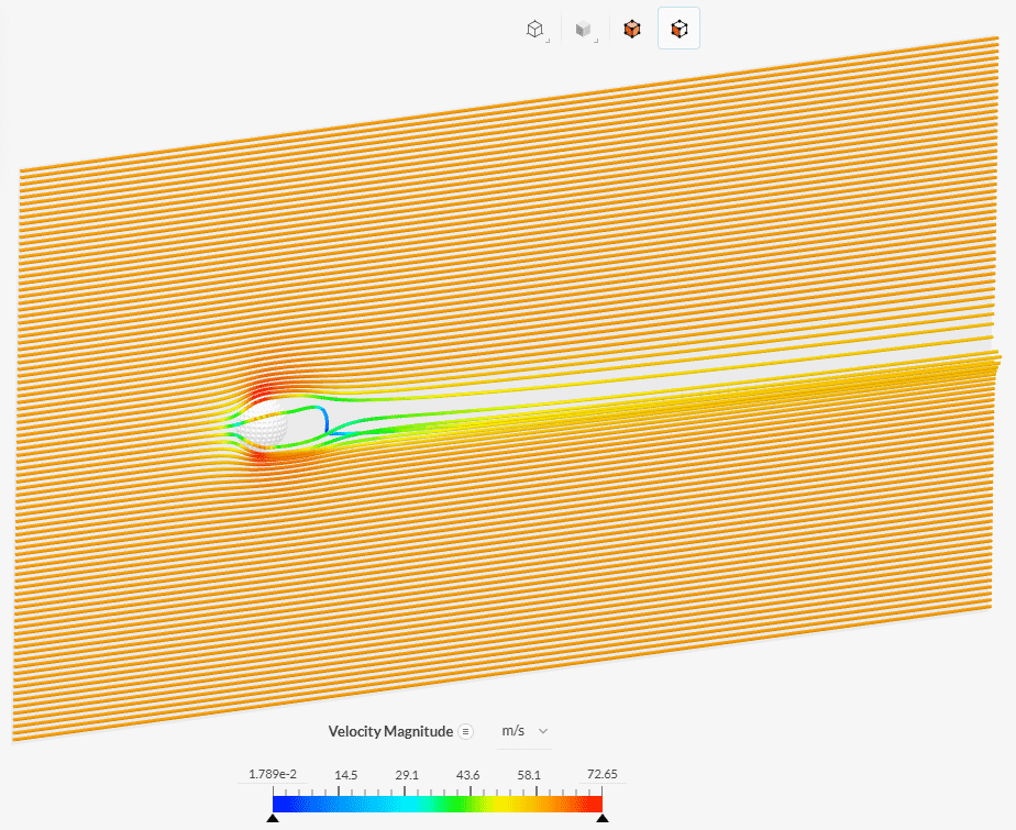
In Figure 46, the behavior of the flow can be observed. The decrease in velocity is obvious in the downstream, where low pressure was previously noticed (Figure 43). Towards the end of the domain, the streamlines gradually tend to become parallel again, reaching ambient conditions.
Animations can be started by choosing ‘Animation’ from the Filters panel:

Click the play button to start the animation. Below is an example of animating the streamlines, colored with the velocity magnitude:

For more information, have a look at our post-processing guide to learn how to use the post-processor.
Congratulations! You finished the tutorial!
Note
If you have questions or suggestions, please reach out either via the forum or contact us directly.
References
Last updated: April 4th, 2026
We appreciate and value your feedback.
Sign up for SimScale
and start simulating now