Validation Case: Laminar Pipe Flow

The aim of this test case is to validate the following parameters of incompressible steady-state laminar fluid flow through a pipe:

Velocity
Pressure drop

The simulation results of SimScale were compared to the analytical results obtained using the Hagen-Poiseuille equations$^1$. The mesh was created with the Hex-dominant Automatic algorithm on the SimScale platform.

View Project

Geometry

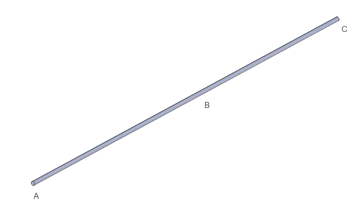
A straight cylindrical pipe was chosen as the flow domain (see Figure 1). Faces A, B, and C represent the inlet, wall, and outlet respectively.

Dimension	Length	Diameter
Value $[m]$	1	0.01

Table 1: Dimensions of the pipe geometry

Analysis Type and Mesh

Tool Type: OpenFOAM®

Analysis Type: Incompressible steady-state analysis.

Turbulence Model: Laminar flow

Mesh and Element Types:

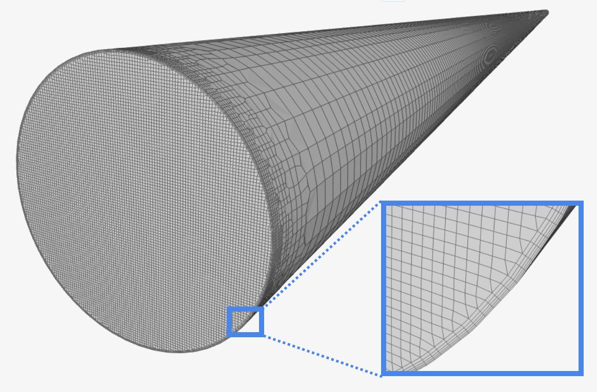
Three structured hexahedral meshes are generated on the SimScale platform using the Hex-dominant Automatic algorithm (see Figure 2). The meshes are gradually refined with a growth rate of 1.25. Later, these meshes are used to verify the mesh independence of the results.

Cell size at the inlet face is smaller than in the other regions. The purpose of this extra measure is to capture the parabolic velocity assignment at the inlet. This topic will be explained in more detail in the next section.

The global cell size and refinement sizes are defined as follows:

Mesh Name	Global Cell Size $[m]$	Surface Refinement – Cylindrical Surface $[m]$	Surface Refinement – Inlet Surface $[m]$	Number of cells [M]
Coarse Mesh	0.0016	8.00E-04	1.00E-04	0.435
Moderate Mesh	1.12E-03	5.60E-04	7.00E-05	0.837
Fine Mesh	7.84E-04	3.92E-04	4.90E-05	1.700

Table 2: Maximum edge length assignment in each mesh and their corresponding refinements

snappy hex mesh used for circular pipe — Figure 2: Coarse mesh used for the SimScale case

Simulation Setup

Fluid:

Water:
- $(\nu)$ Kinematic viscosity = 10^-6 $\frac{m^2}{s}$

Boundary Conditions:

One of the parameters of interest, which is the topic of this validation case, is the pressure drop through the pipe. Above all, the Hagen–Poiseuille equation considers the flow at the inlet to be fully developed. There are two common CFD methods to generate a fully developed flow:

Method 1: Firstly, approximate the laminar entry length. Then extend the pipe inlet by adding the entry length. The flow becomes fully developed after the entry length is achieved. As a result, this measure ensures the correct velocity profile at the pressure measure points. As a simple approximation, you may consider the entry length as 138 times the pipe diameter. Similarly, more complex empirical equations with Reynolds number are available in the literature.
Method 2: At the inlet, define a parabolic velocity profile, which matches with the Hagen-Poiseuille parabolic velocity equation.

The first method is impractical since it will require a significantly higher mesh count and so the computation resources. Therefore, the parabolic velocity input option is preferred in this project.

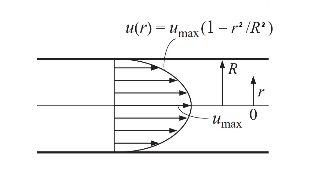
The parabolic velocity profile through a circular pipe in a laminar flow is approximated as follows:

$$ u_z = u_{z\ max} (1-{r^2 \over R^2}) $$

$$ u_ {z\ max} = 2 \ u_{z\ avg} $$

where $ u_z $ is the z-component of the velocity along the axis, $u_{z\ avg}$ is the average inlet velocity, $u_{z\ max}$ is the maximum velocity that occurs at the centerline, $r$ is the radial distance from the centerline, and $R$ is the radius of the circular pipe$^2$. For instance, a parabolic velocity profile in a circular pipe is illustrated in Figure 3.

fully developed laminar pipe flow hagen poiseuille — Figure 3: Schematics for a fully developed laminar flow velocity profile in a circular pipe $^2$

The following boundary conditions are applied to the corresponding pipe surfaces:

Face	Boundary type	Value
Inlet (A)	Velocity inlet	Fixed value of $2 \times 0.1 \times (1-(((x)^2+(z)^2)^{0.5/0.005})^2)$ $m/s$ in the y-direction
Outlet (C)	Pressure outlet	Fixed value of 0 $Pa$
Wall (B)	Wall	No-slip

Table 3: Summary of boundary conditions

Results

Pressure drop results per mesh are summarized in Table 4:

Mesh Name	Number of cells [M]	Pressure Drop $[Pa]$
Coarse Mesh	0.435	32.192
Moderate Mesh	0.837	32.156
Fine Mesh	1.700	31.993

Table 4: Mesh sensitivity study

Pressure results change less than 1% between the meshes. Although the coarse mesh result seems reasonable, fine mesh results must be more accurate. Therefore, the results of the fine mesh are presented in this study.

The analytical solution gives us the following equations for maximum axial velocity, pressure drop and developed radial velocity profile:

$$u_{z \ max} = 2u_{z \ avg}$$

$$\Delta P = \frac{128}{\pi} \frac{\mu L}{D^4} Q $$

$$u_z = -\frac{1}{4\mu} \frac{\partial p}{\partial z}(R^2 – r^2)$$

where,

$ u_{z\ avg} $: Average inlet velocity $[m/s]$
$ u_{z\ max} $: Maximum velocity that occurs at the centerline $[m/s]$
$ u_{z} $: Velocity along the axis $[m/s]$
$r$: Radial distance from the centerline $[m]$
$R$: Radius of the circular pipe $[m]$
$\Delta P$: Pressure loss $[Pa]$
$\mu$: Dynamic viscosity $[kg/(m\cdot s)]$
$L$: Length of circular pipe $[m]$
$D$: Diameter of circular pipe $[m]$
$Q$: Volumetric flow rate $[m^3/s]$
$\frac{\partial p}{\partial z}$: Pressure gradient along the pipe $[Pa/m]$

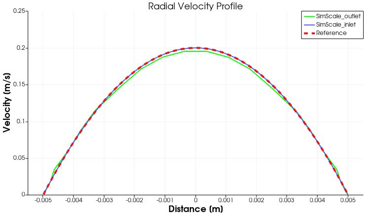
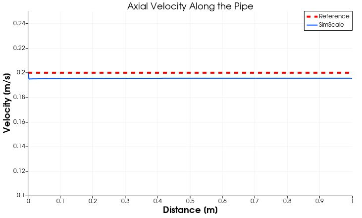
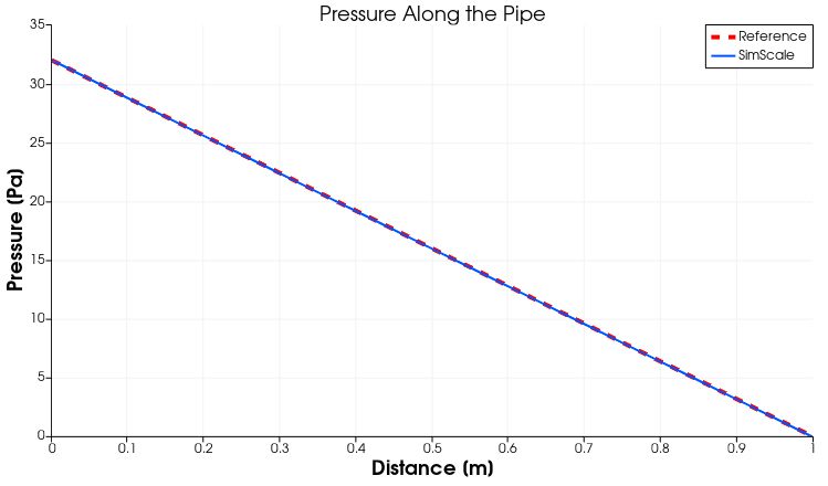
A comparison of the velocity and pressure drop obtained with SimScale with analytical results is given in Figures 4A, 4B, and 4C. Figure 4A shows the developed radial velocity profile at the inlet and the outlet.

References

- Hagen–Poiseuille flow from the Navier–Stokes equations
- Çengel, Yunus A. Heat Transfer: A Practical Approach. Boston, Mass: WBC McGraw-Hill, 1998.
Last updated: July 30th, 2025
Did this article solve your issue?
How can we do better?
We appreciate and value your feedback.