Tutorial: Linear Static Analysis of a Wheel Loader Arm

This article provides a step-by-step tutorial for a linear static analysis of a Wheeled Loader Arm.

wheel loader arm post processing report image header — Figure 1: Post-processing contours on a Wheeled Loader Arm.

This tutorial demonstrates the process of setting up and executing a linear static analysis on a wheel loader arm using SimScale. The steps covered follow the standard SimScale simulation workflow and include:

CAD Preparation – Import and prepare the geometry
Simulation Setup – Define physics, materials, and boundary conditions
Meshing – Generate the mesh using the default settings
Simulation Run – Execute the simulation
Post-Processing – Analyze and visualize the results

Objectives

Throughout the tutorial, the following tasks will be performed:

Apply boundary conditions, materials, and other simulation properties
Generate the mesh using SimScale’s standard meshing algorithm
Visualize the resulting stress field
Apply solid color visualization for volume rendering
Create a safety factor field
Measure displacements at a specific control point

1. Prepare the CAD Model and Select the Analysis Type

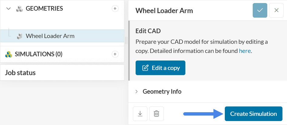
Begin by selecting the button below. This action copies the tutorial project, including the geometry, into the SimScale Workbench for further setup and simulation.

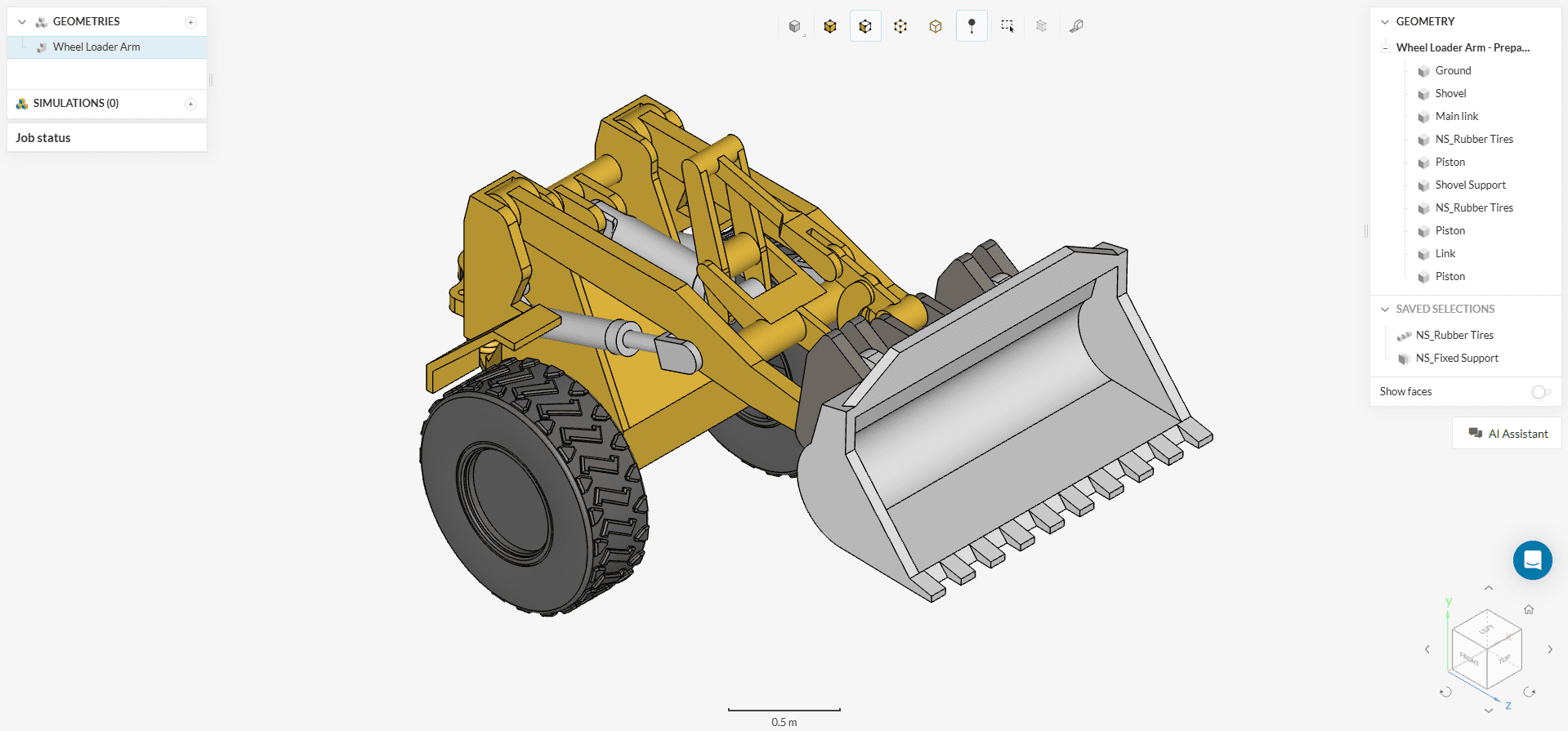
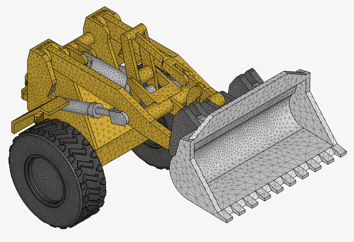
Import tutorial into the Workbench

Once the tutorial project is imported, the Workbench will display an empty simulation setup along with the geometry. The image below illustrates the expected view after the import is complete.

wheel loader arm geometry in the workbench — Figure 2: Overview of the Workbench after importing the Wheeled Loader tutorial base project.

1.1 Create the Simulation

To begin the simulation setup, use the ‘Create Simulation’ button located in the geometry dialog box. This opens the simulation creation panel where analysis types can be selected.

geometry dialog box showing how to create a new simulation run in simscale — Figure 3: Geometry dialog box.

At this stage, the simulation type selection panel appears, allowing the choice of the desired analysis type from the available options.

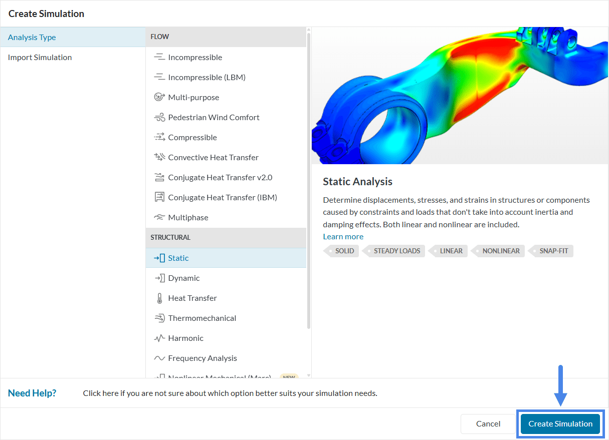
simscale simulation library showing selection for static simulation — Figure 4: SimScale supports a wide range of physics. This tutorial consists of a **‘Static’** analysis.

Select the ‘Static’ analysis type for this simulation.

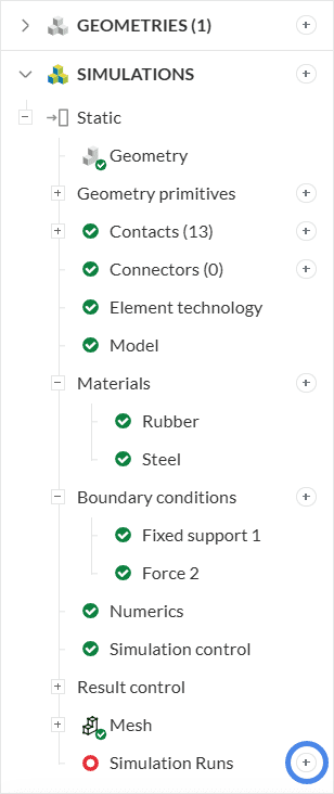
The platform then displays the simulation tree, which lists all settings that must be defined before running the analysis.

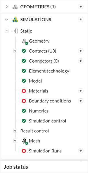
simulation tree of a linear static simulation in simscale — Figure 5: New simulation tree

The setup for the linear static analysis of the wheel loader arm can now begin.

2. Simulation Settings

Before running the simulation, define the following key settings:

Contacts between different parts of the assembly
Gravity direction to simulate the effect of weight
Materials assigned to the tires and components of the wheel loader
Boundary conditions to reflect physical constraints and loads

2.1 Contact Settings

The first tab to configure is ‘Contacts’. Since the geometry was prepared according to best practices, all relevant faces are in direct contact in the CAD model. As a result, SimScale automatically assigns bonded contacts between touching faces when the geometry is added to the simulation.

The only required adjustment is to enable the ‘Allow node merging’ option. This setting ensures a continuous stress field across the entire assembly, leading to improved accuracy in contact modeling.

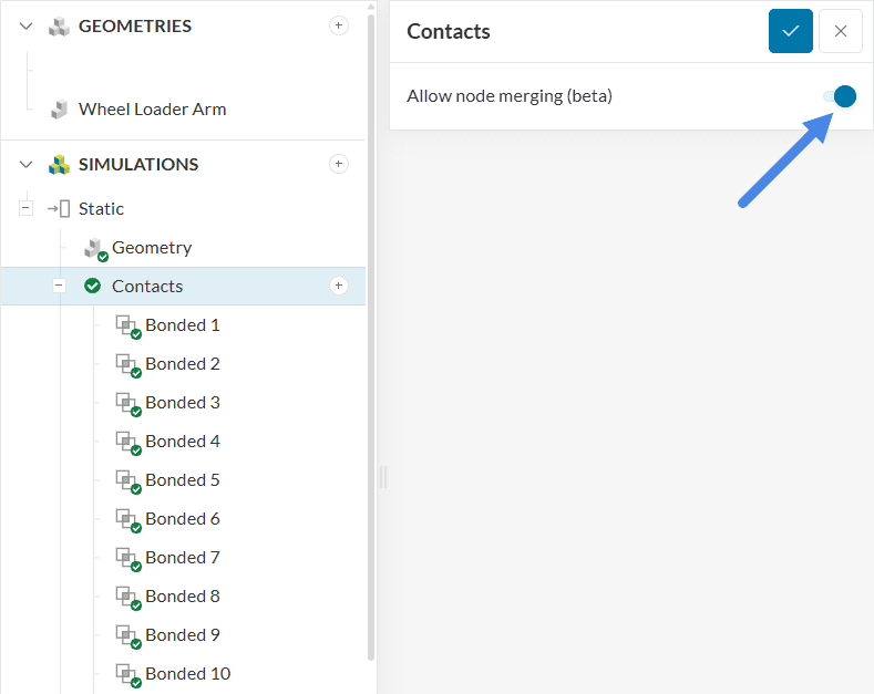
node merging contact settings — Figure 6: Enabling node merging under Contact settings

Note that this simulation uses only bonded contacts, which are of the linear kind. Bonded contacts assume a perfect connection between the selected surfaces, meaning no relative motion is allowed at the interface. The corresponding nodes on both surfaces share the same displacement, effectively creating a rigid connection between the parts in the context of the linear static analysis. To learn more about linear contacts, please check the relevant documentation.

2.2 Direction of Gravity

The gravity direction and magnitude significantly influence the simulation results, as the weight of the wheel loader arm contributes substantially to the overall load. Define gravity settings by selecting ‘Model’ from the simulation tree.

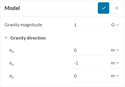
gravity setting simscale wheel loader — Figure 7: Gravity settings are defined based on the orientation cube.

In this setup, gravity is defined with a magnitude of 1 g (equivalent to 9.81 m/s²) and acts in the negative y-direction.

2.3 Define a Material

The material for the different parts in the wheel loader arm assembly must also be defined. To select a material, click on ‘Materials’ in the simulation tree. This action opens the solid materials library, as shown in the image below.

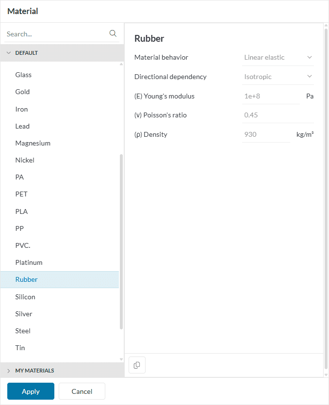
material library of simscale and rubber is selected for static linear simulation — Figure 8: SimScale’s solid materials library

Begin by assigning material to the tires. Select ‘Rubber’ from the materials library and confirm the selection by clicking ‘Apply’. Then, use the assignment box to select the appropriate volumes. The tires can be found in the right-hand panel under ‘Saved Selections’.

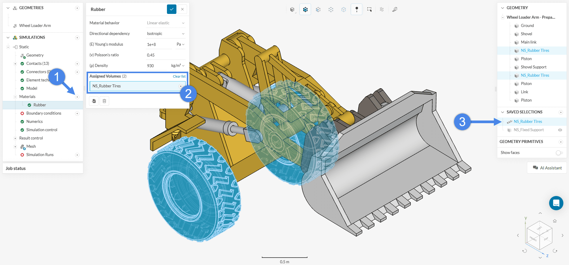
Assign rubber material simscale — Figure 9: Rubber material assigned to the tires of the Wheel Loader Arm model

Click the check icon to save the material assignment.

Next, define the material for the remaining components of the assembly. Create a new material, then hide the rubber tires by clicking the eye icon in the right-hand panel. To assign the material, either:

Right-click anywhere in the Workbench and choose ‘Assign all’, or
Manually select all parts of the geometry except for the tires and assign the material.

assign steel material wheel loader simscale — Figure 10: Steel material assigned to the remaining parts of the Wheel Loader Arm model

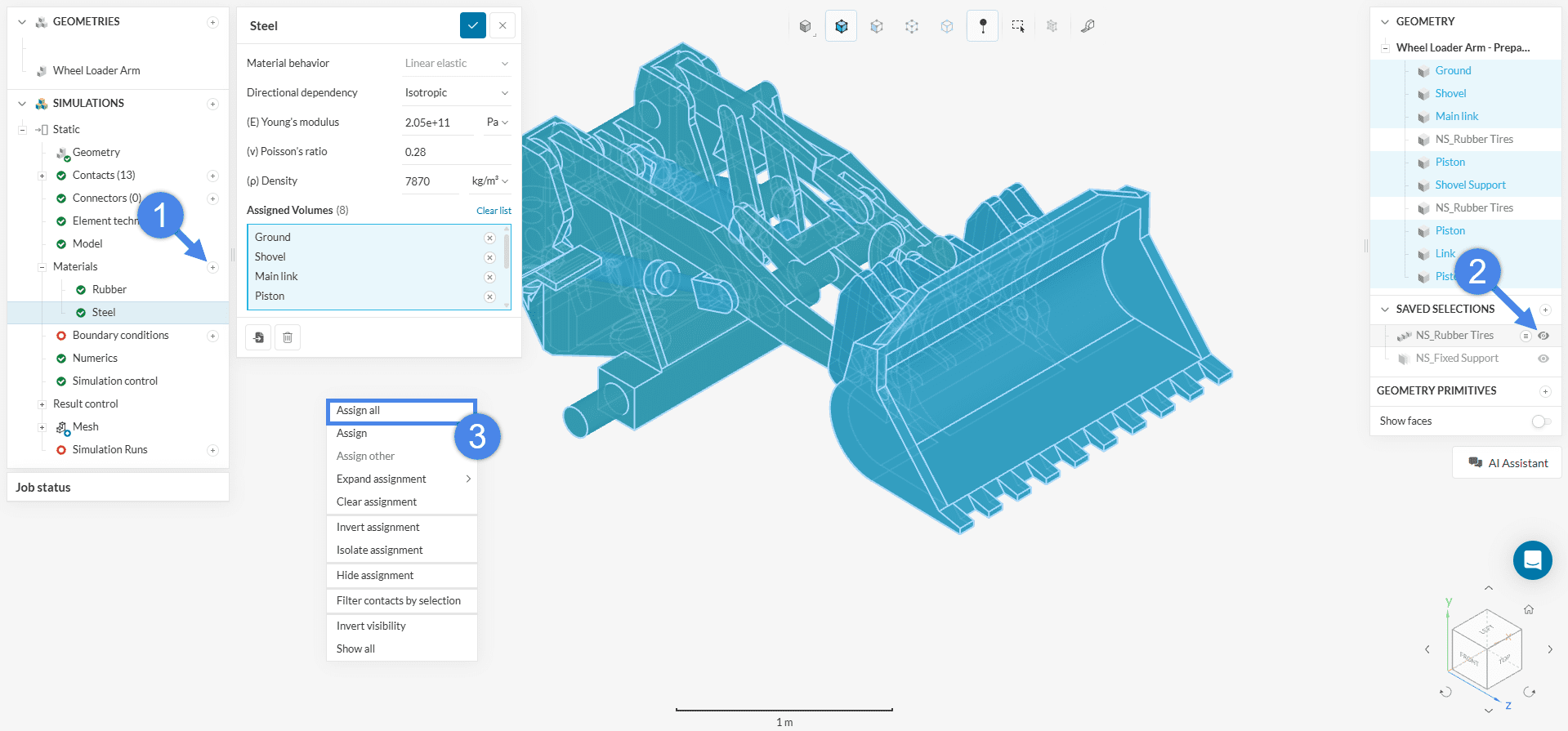
Custom materials can be defined by adjusting the material properties manually. It is also possible to assign a custom name to the material for easier identification within the project.

2.4 Assign the Boundary Conditions

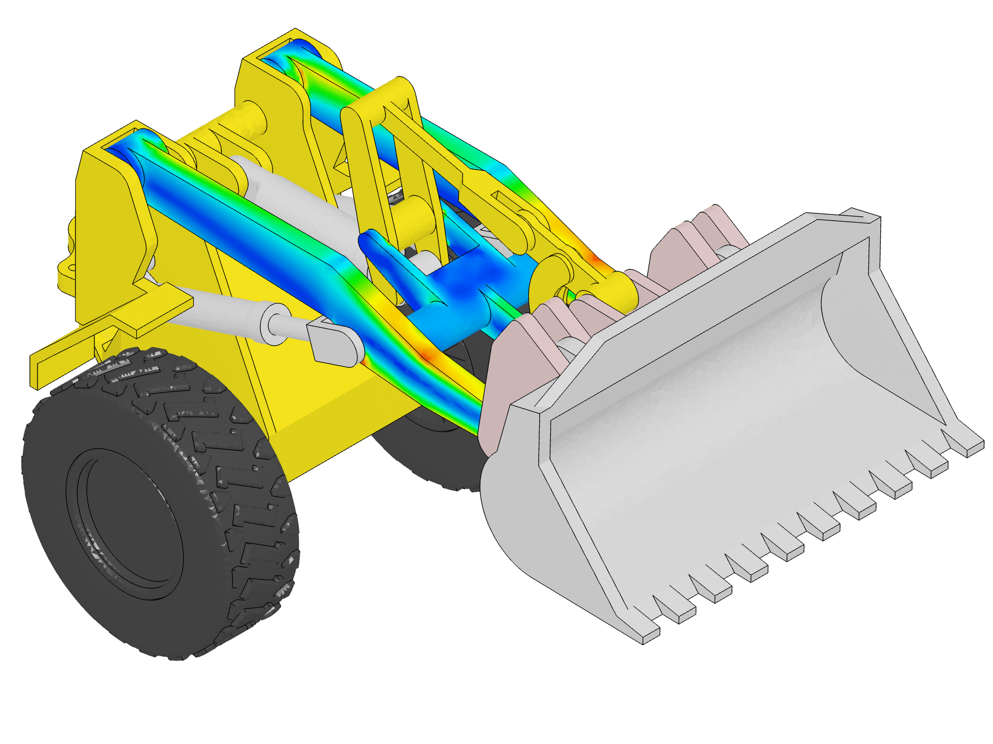
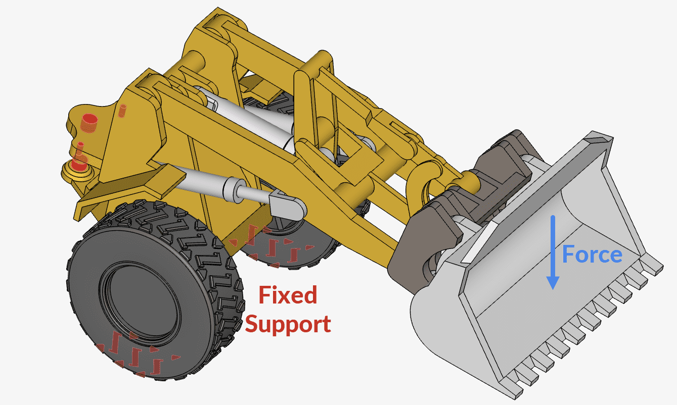
Boundary conditions are essential for accurately simulating real-world behavior. They define the physical constraints and loads applied to the design. In this simulation, both ‘Fixed support‘ and ‘Force‘ boundary conditions are used. The image below provides an overview of the setup and physics involved.

boundary conditions that are used for linear static simulation on a wheel loader arm — Figure 11: Boundary conditions overview for this simulation

The following steps describe how to assign each boundary condition required for the simulation.

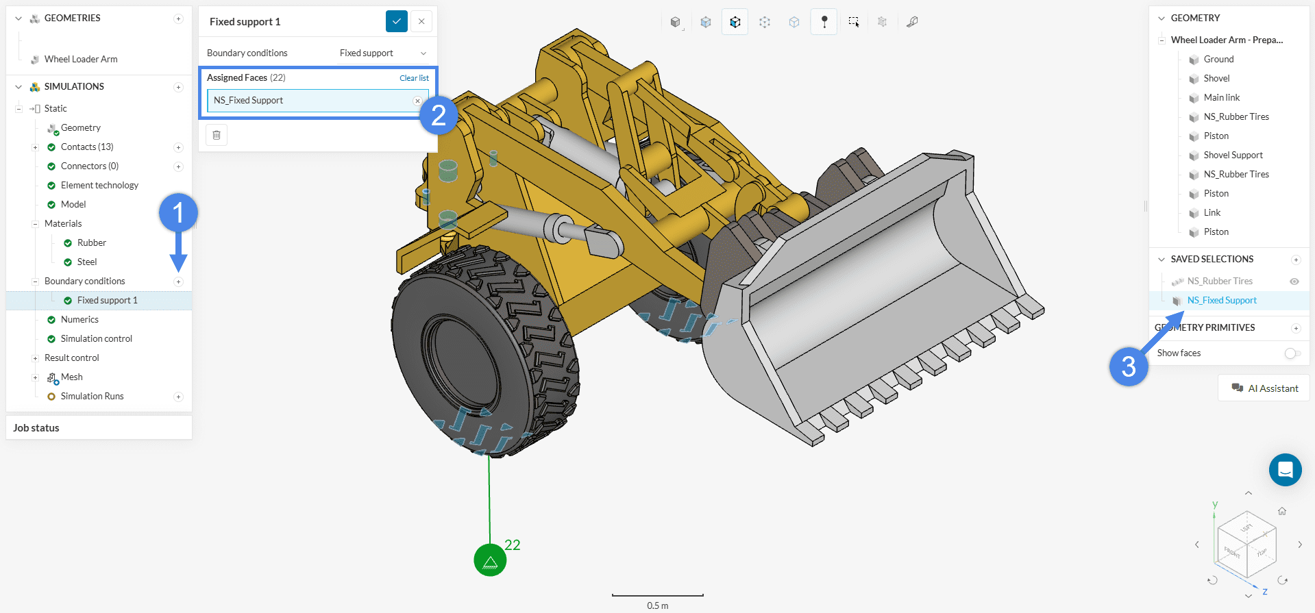
a. Fixed Support

To define the first boundary condition, click the ‘+’ button next to ‘Boundary conditions’. From the list of options, select ‘Fixed support’. In the ‘Assigned faces’ section, open the selection box and choose the NS_Fixed Support entry from the ‘Saved Selections’ panel.

steps to select fixed support boundary condition for linear static simulation — Figure 12: Fixed support boundary condition assignment

b. Force

Repeat the same process to create a ‘Force’ boundary condition. Click the ‘+’ button next to ‘Boundary conditions’, select ‘Force’ from the list, and proceed with the required assignments.

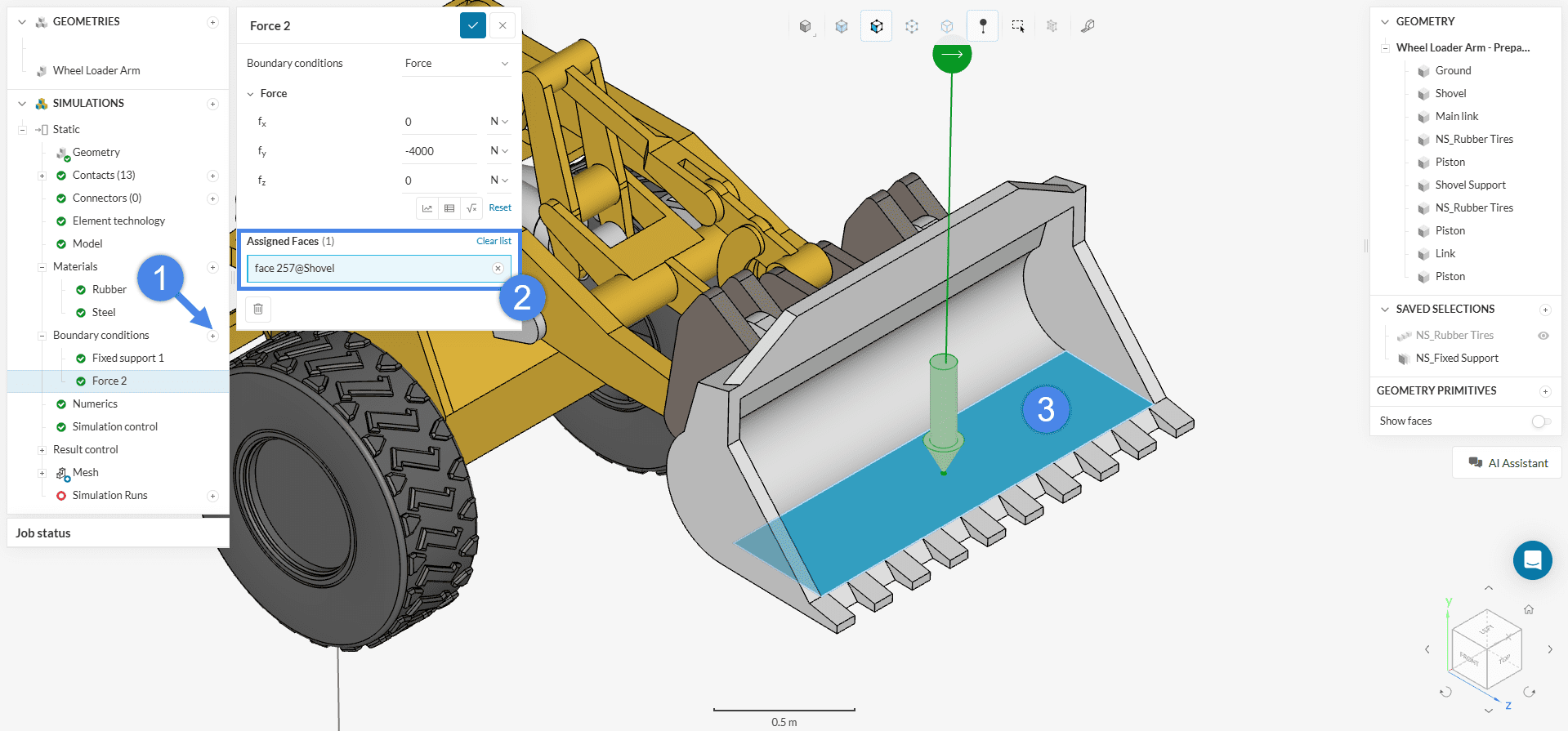
-4000 n force boundary conditon applied at the shovel of a wheeled loader arm for a linear static simulation — Figure 13: Force boundary condition, taking into account the orientation cube.

Define the force as –4000 N in the y-direction, based on the orientation indicated by the cube in the viewer.

2.5 Result Control

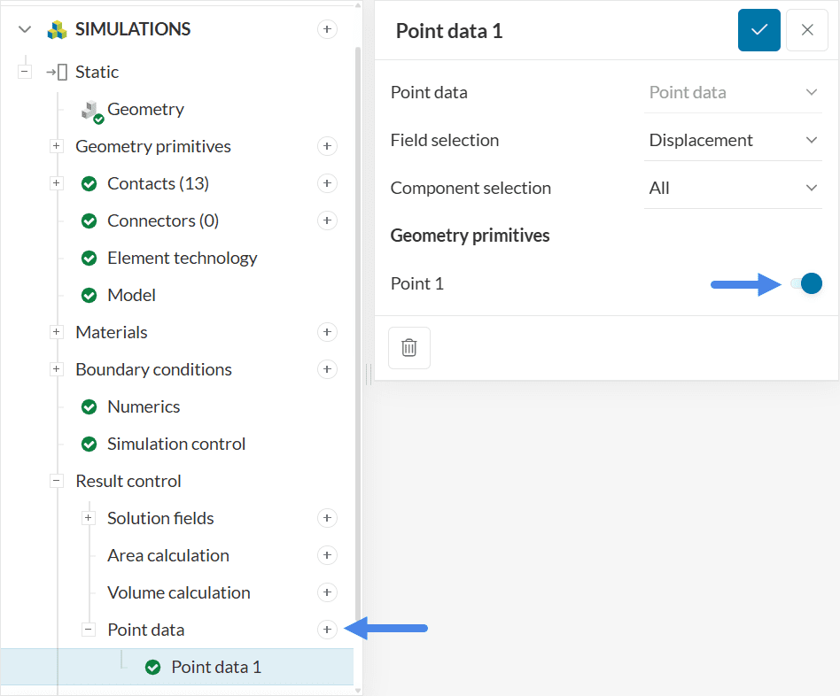
Displacement at a specific point is a key result in static analyses. To monitor this quantity, create a result control at the desired location.

Begin by creating a point geometry primitive via ‘Geometry Primitives’ > ‘Point’. Use the ‘Pick from Viewer’ option to select a point on the surface of the wheel loader arm. This point will serve as the reference for the displacement measurement.

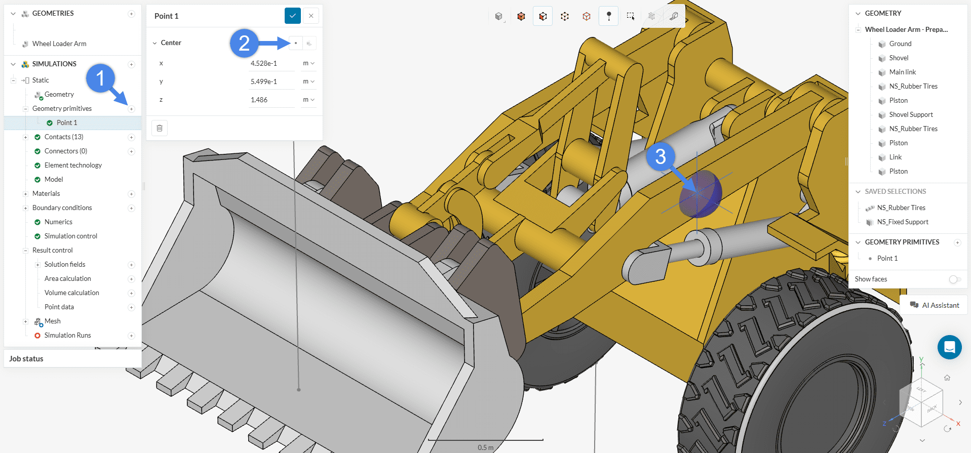
how to create a point geometry primitive — Figure 14: Create a point geometry primitive and pick the location from the viewer

Next, navigate to ‘Result Control’ > ‘Point data’ and create a new control item. Assign it to the previously defined ‘Point 1’ to track the displacement at that location.

create a point data result control — Figure 15: Assign a new Point data to the created Point geometry primitive

The displacement results for each spatial direction can be accessed under Completed run > ‘Point data’ once the simulation finishes.

Note

No changes were made for the Numerics and Result control settings for this tutorial as default settings will be sufficient.

3. Mesh

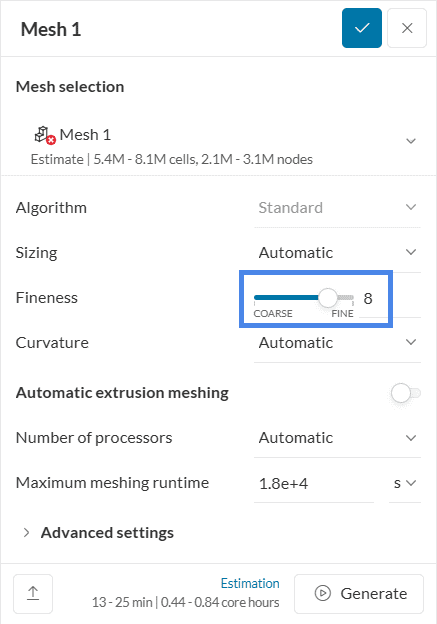
To generate the mesh, use the ‘Standard’ meshing algorithm, which is automated and typically provides good results for most geometries.

For this simulation, adjust the fineness level to 8 instead of the default value of 5. In linear static simulations, SimScale automatically creates second-order meshes, which enhance the accuracy of the analysis.

mesh settings wheeled loader tutorial — Figure 16: Mesh dialog box

Why 2nd Order Elements?

Second-order elements are generally recommended for static analyses due to their improved accuracy in capturing deformation and stress gradients. For more details, refer to the article: Which type of finite element should I use?

The mesh order can be specified under the Element Technology tab in the simulation tree. More information is available here: Element Technology

The resulting mesh appears as shown below, illustrating the geometry discretized with second-order elements and a fineness level of 8.

mesh of a wheel loader using the standard meshing algorithm in simscale — Figure 17: Mesh of the Wheel Loader Arm model

4. Start the Simulation

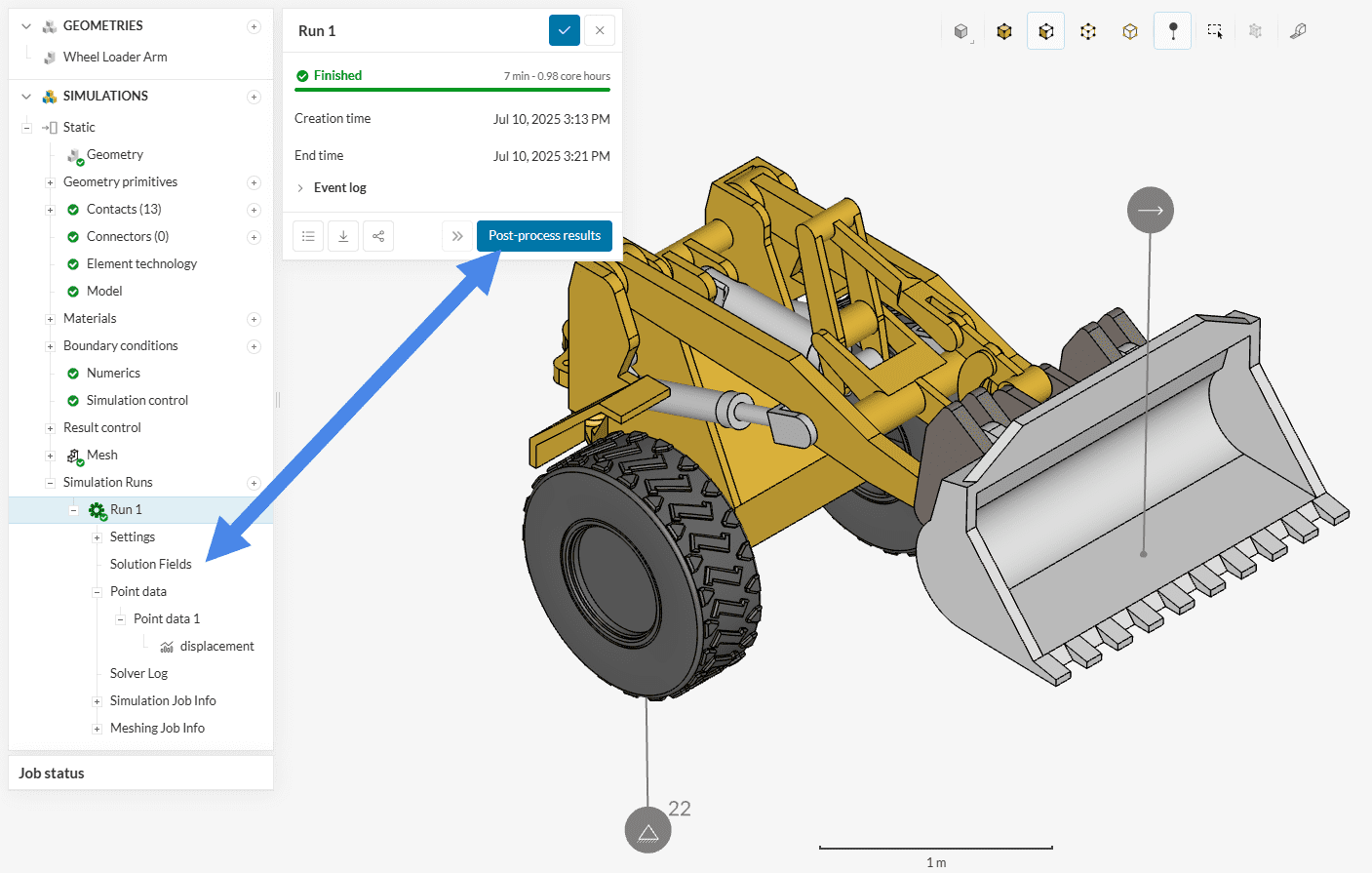
To start the simulation, click the ‘+’ button next to ‘Simulation Runs’ in the simulation tree. This initiates a new run using the defined setup and mesh.

simulation tree of simscale with steps on how to start a new simulation run — Figure 18: Steps to start a new simulation run.

A dialog box appears displaying an estimate of the computing resources required to run the simulation. Proceed by clicking ‘Start’ to begin the simulation run.

5. Post-Processing

Once the simulation run finishes, results can be accessed in one of the following ways:

Click on ‘Solution fields’ under the simulation run, or
Click on the ‘Post-process results’ button in the run dialog.

access online post-processor linear static analysis wheeled loader arm — Figure 19: The two ways to access the online post-processor in SimScale

In the post-processing environment, analysis of the simulation results can begin. This tutorial focuses on the following post-processing tasks:

Visualizing the von Mises stress field
Changing the volume rendering to solid colors instead of result fields
Creating a safety factor field
Reviewing the result control data for displacement at the defined point

5.1 Von Mises Stress

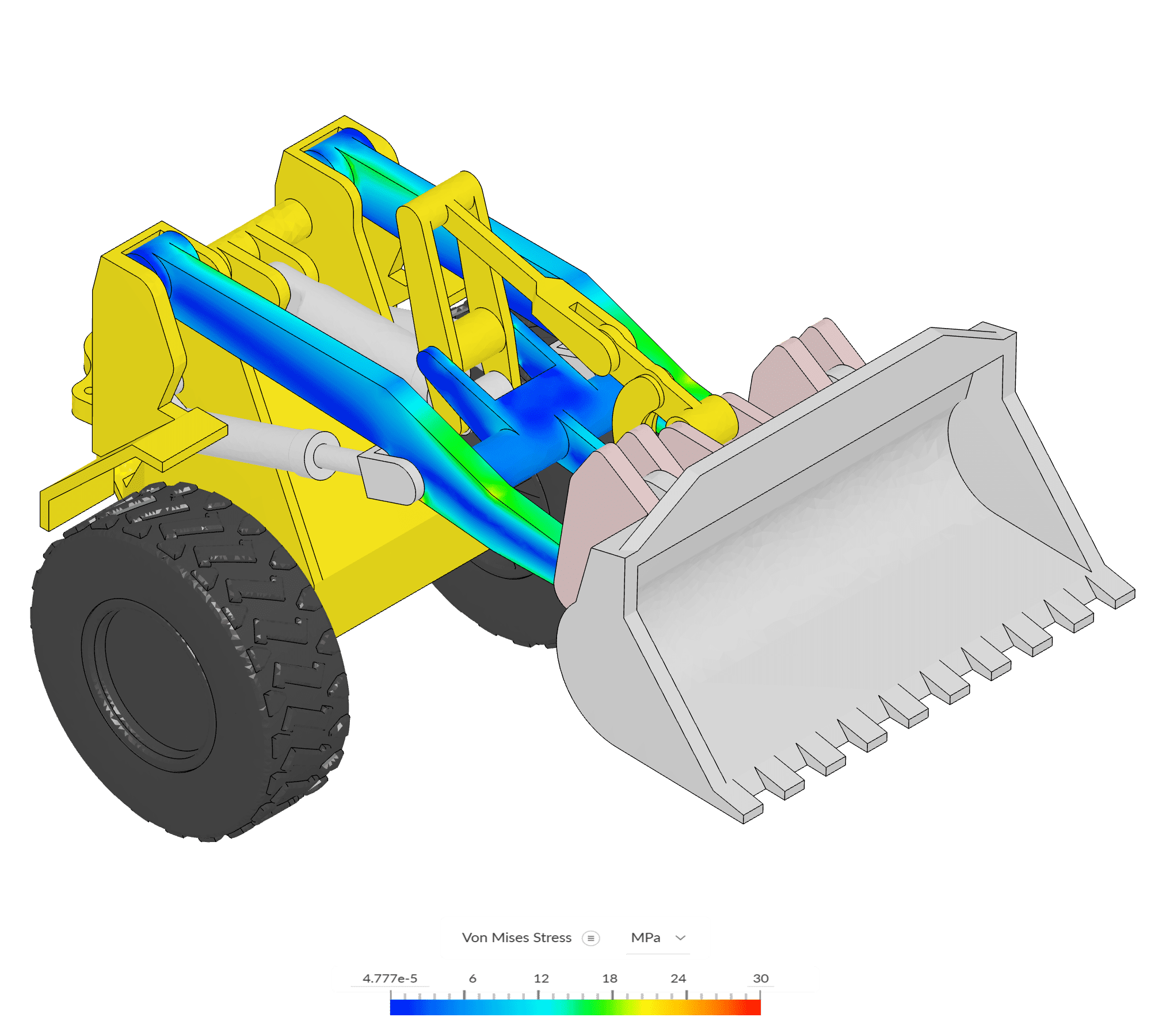
To analyze the von Mises stress on the wheel loader arm:

Set ‘Parts Color’ to von Mises Stress in the post-processing panel
Change the stress units from Pa to MPa for improved readability
Adjust the upper threshold of the color legend to 30 MPa to enhance contrast and detail in the stress distribution

von mises stress wheel loader arm adjust legend limits — Figure 20: Von Mises stress distribution in the Wheel Loader Arm due to the applied loads

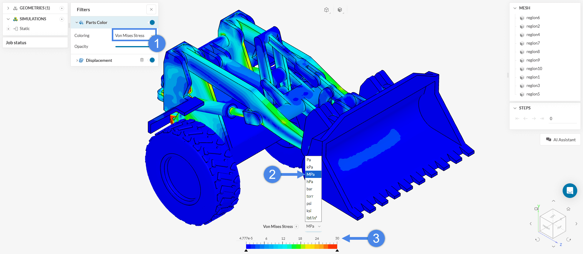
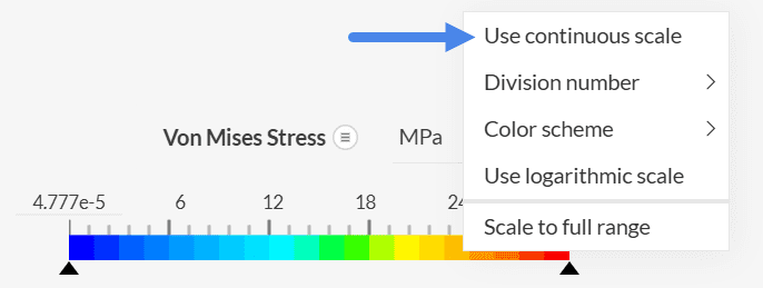
When stress gradients are clearly visible, switching to a continuous scale provides a smoother and more accurate visualization. To enable this, right-click on the legend and select Use continuous scale.

use continuous scale legend post processor — Figure 21: Change the scale from stepped to continuous

Volume color customization

For improved visual clarity or to generate presentation-ready images, volume colors can be customized in the post-processor.

To change the color of specific volumes:

Select the desired volumes
Right-click and choose ‘Edit color’
Pick a preferred color from the palette

The example below illustrates this feature applied to the tires.

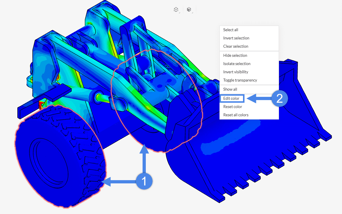
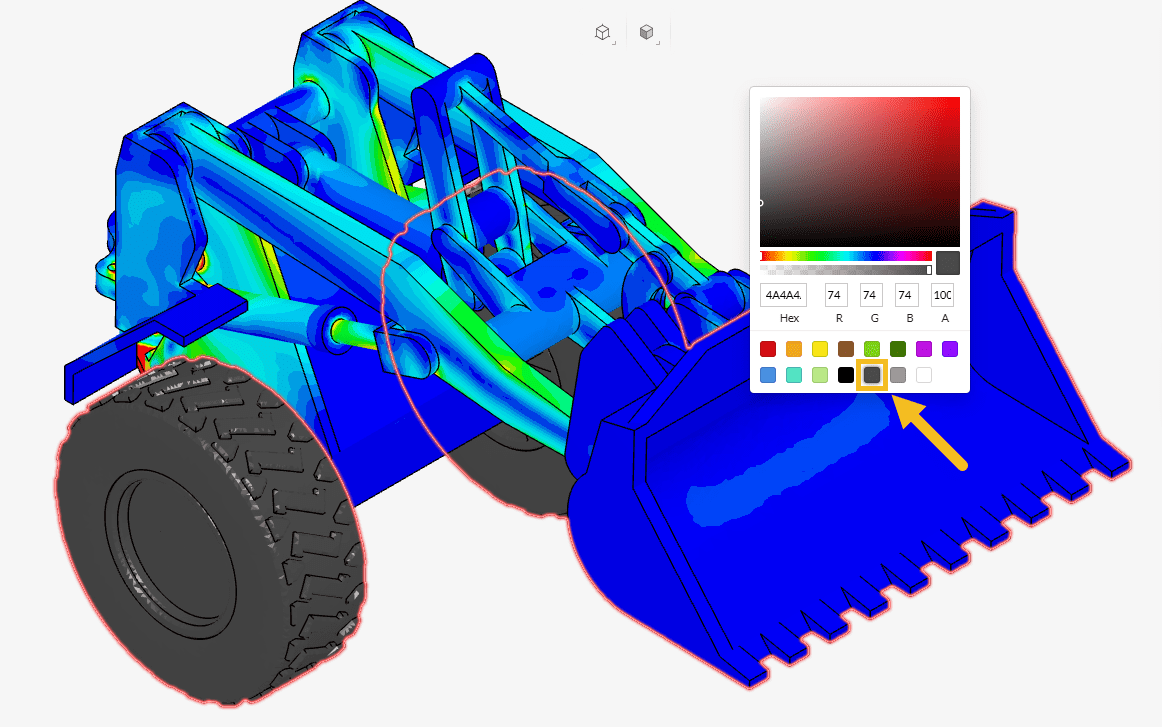
select parts and edit color post processor — (a) Select parts > Right-click > Edit color

assign solid color to specific parts post-processor — (a) Select parts > Right-click > Edit color

Figure 22: How to assign a solid color to individual parts in the Wheel Loader Arm assembly

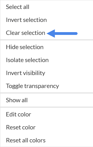
To assign a solid color to additional parts:

Right-click anywhere in the viewer and select ‘Clear selection’
Select the new volumes to be edited
Right-click and repeat the ‘Edit color’ workflow as previously described

This process can be repeated for each group of parts requiring a different solid color.

clear selection to assign solid color to other parts in post processor — Figure 23: After each solid color assignment, right click in the workbench and ‘Clear selection’

Final visualization

After adjusting the legend, configuring the field display, and applying the desired solid colors, the von Mises stress field becomes clearly visible while highlighting the Main Link component.

stress results linear static analysis wheel loader arm — Figure 24: Von Mises stress distribution, highlighting the Main Link

5.2 Create a Safety Factor Visualization

An important result in structural analysis is the Safety Factor field, which provides insight into how close the structure is to failure. It is calculated as:

$$ S_f = \frac{\sigma_y}{\sigma_{vm}} $$

where:

is the material yield strength
is the von Mises stress

This field can be created using the ‘Field Calculator‘ in the post-processor, as illustrated in Figure 25.

To visualize the safety factor:

Enable the new field in the legend
Adjust the legend limits for better contrast
Right-click the legend and select the ‘Normal inverted’ color scheme, which highlights lower (more critical) values more effectively

crate safety factor field using the field calculator simscale — Figure 25: Set up a Safety factor field by using a Field Calculator

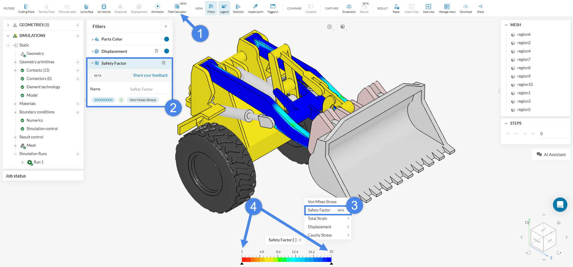
Below are key considerations when using the ‘Field Calculator’ in the post-processor:

Press Enter after each input (numbers, operators like +, -, *, /, parentheses, fields such as Von Mises Stress, or functions like abs, sqrt to apply it to the expression.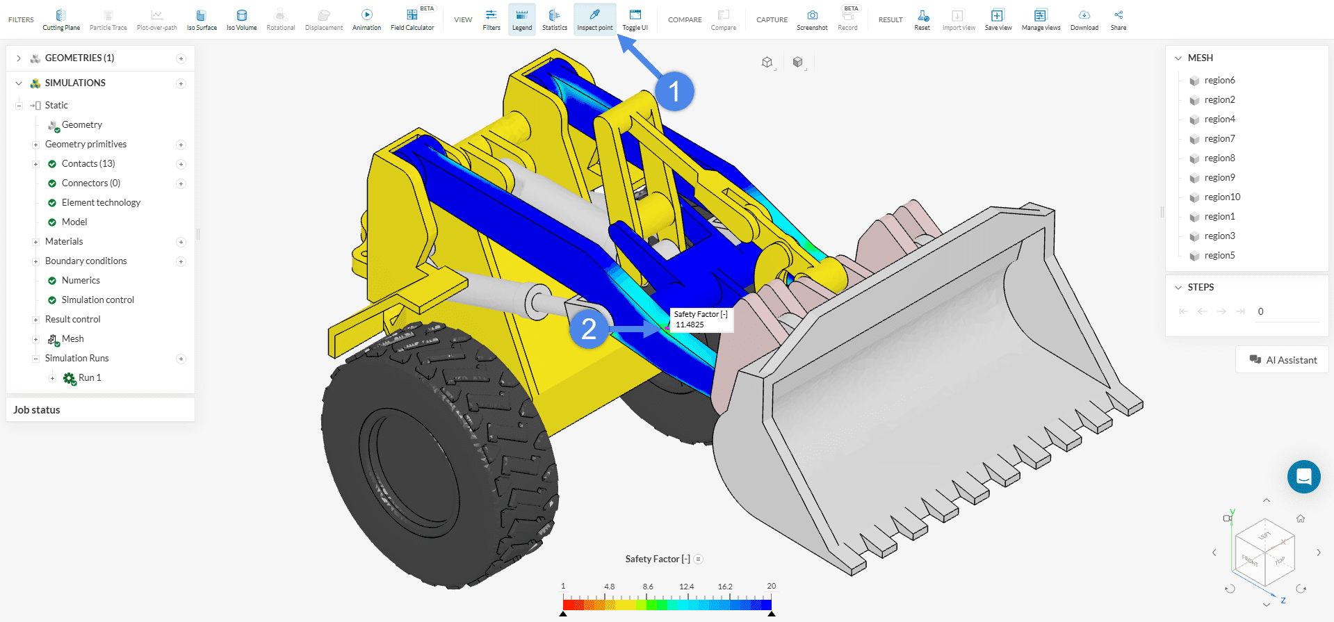
All inputs must use SI units. For stress, this means working in Pascals (Pa), not MPa or kpsi.
Once a field is created using the calculator, it cannot be edited. To make changes, a new field must be created.
After generating the field and adjusting the visualization, use the ‘Inspect Point’ tool to click on any region of the model and retrieve the corresponding field value.

use inspect point to inspect safety factor at a point — Figure 26: Use the Inspect point tool to inspect the created Safety factor field at a point

5.3 Displacement at the control point

To access the displacement values:

Navigate to ‘Run 1’ > ‘Point data’ in the simulation tree
Click on the result item to visualize a table displaying the displacement components (x, y, z) at the specified control point

visualize the measured displacement for three directins after the run's completion — Figure 27: Retrieving the displacements calculated by the result control item after the Run’s completion

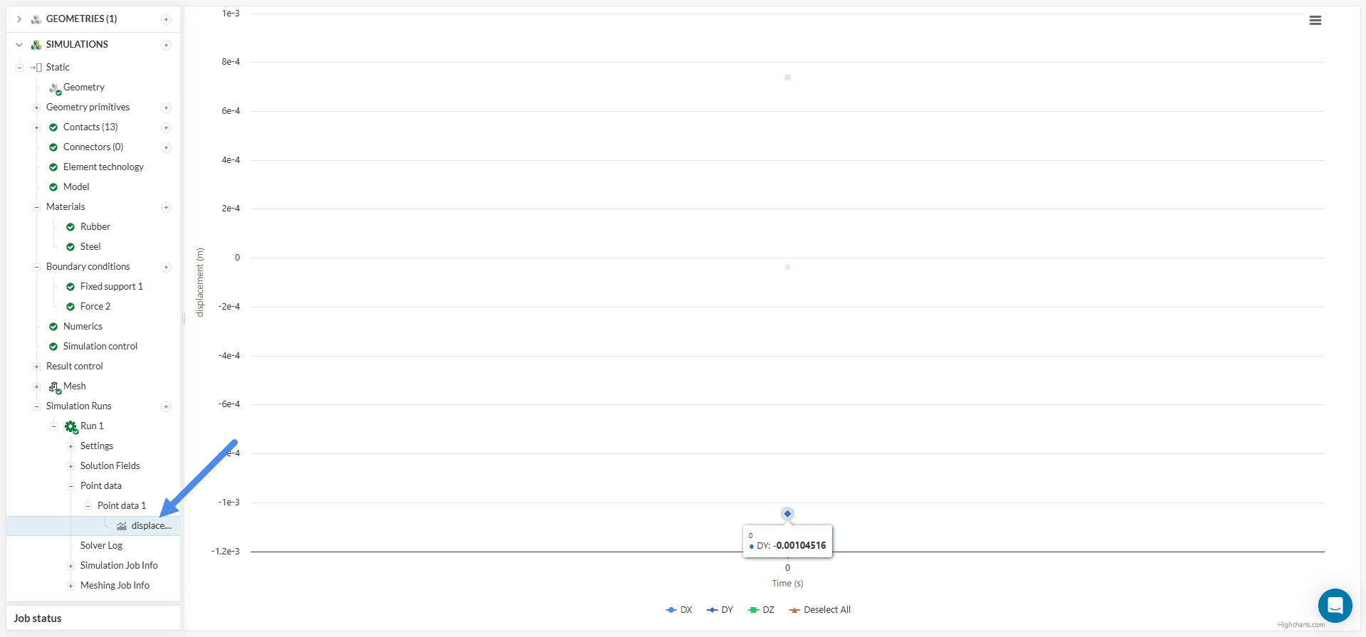
The displacement measured at the control point indicates that the maximum deformation occurs in the y-direction, which aligns with the direction of the applied force. The observed displacement is approximately 1 mm.

Congratulations! You finished the tutorial!

Have a look at the finished project