Advanced Tutorial: Bending of an Aluminium Pipe
This article provides a step-by-step tutorial for performing a nonlinear structural simulation of an aluminium pipe bending process. The objective is to analyze the deformation and stress distribution that develop in the pipe during bending, including nonlinear effects such as material plasticity, physical contact, and large deformations.
This tutorial explains how to:
- Set up and run a nonlinear static simulation.
- Assign boundary conditions, materials, and other simulation properties.
- Mesh the geometry using the SimScale standard meshing algorithm.
- Explore the results with the SimScale online post-processor.
The tutorial follows the standard SimScale workflow:
- Prepare the CAD model for the simulation.
- Set up the simulation.
- Set up the mesh and run the simulation.
- Analyze the results.
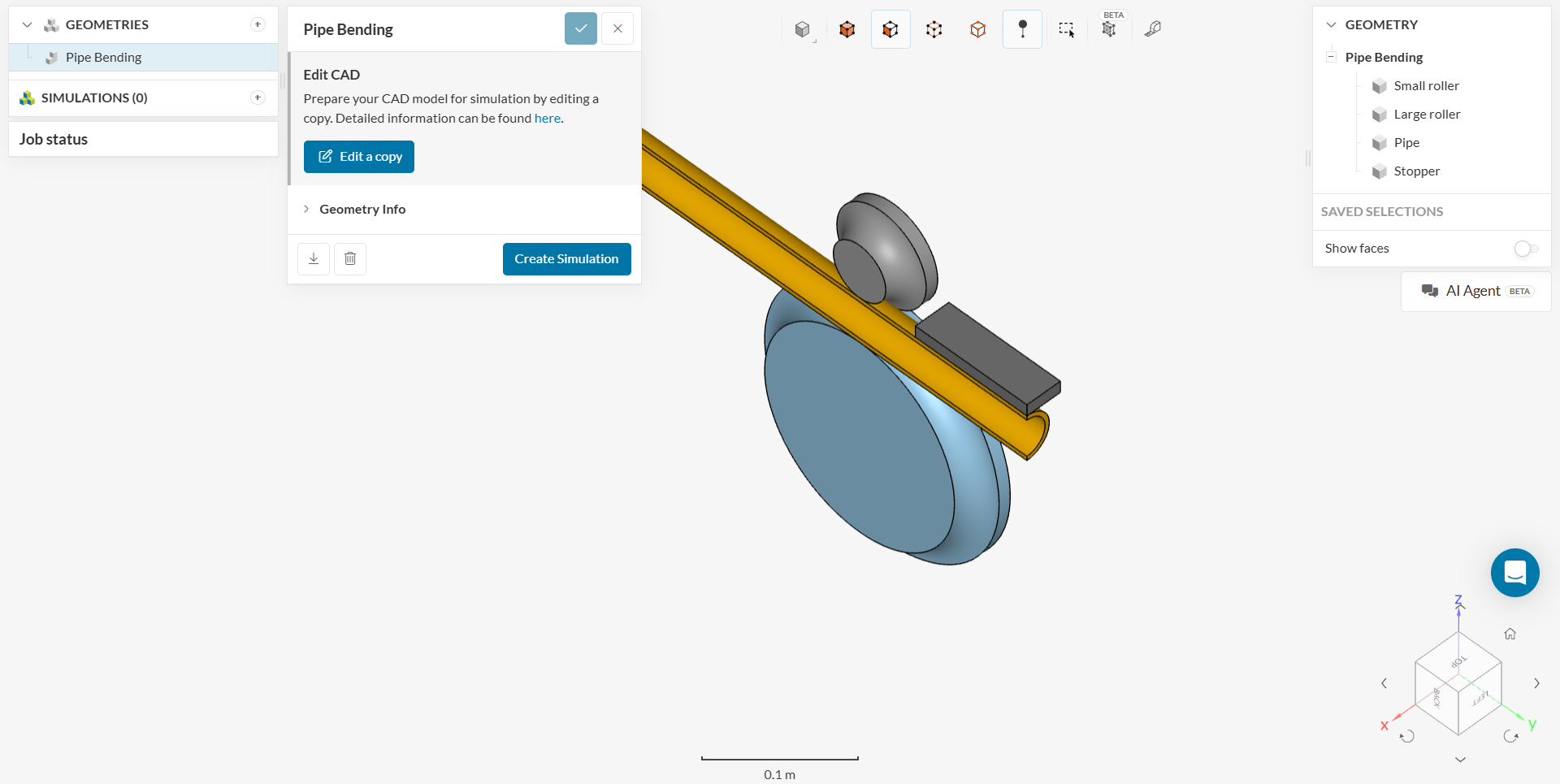
1. Prepare the CAD Model and Select the Analysis Type
Start by clicking the button below. This copies the tutorial project, including the aluminium pipe geometry, into your own workbench.
The image below shows what should be visible after importing the tutorial project.
If you are using your own CAD model, follow these instructions:
All solid geometry should be free of any interference, intersecting surfaces, and small edges. Fix these issues in CAD before bringing the geometry into the SimScale platform. More specific preparation details are mentioned here.
Before starting to set up the model, check the following:
- Make sure that the imported geometry consists of solid parts and not sheet/surface elements.
- If the geometry has small fillets or round faces that are insignificant for the analysis, it is recommended to remove them in CAD. This will dramatically reduce mesh cell count and therefore solve time.
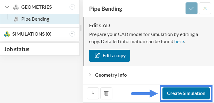
1.1. Create Simulation
To begin the simulation setup, use the Create Simulation button located in the geometry dialog box. This opens the simulation creation panel where analysis types can be selected.
At this stage, the simulation type selection panel appears, allowing the choice of the desired analysis type from the available options.
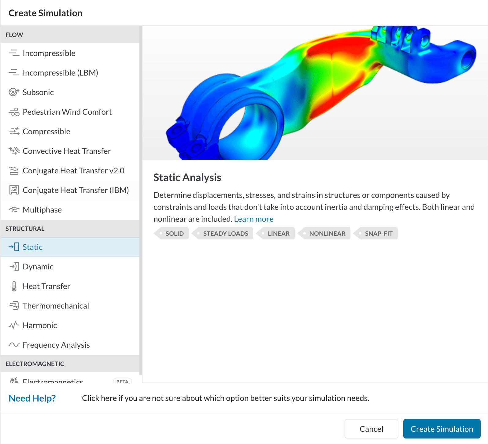
Select Static as the analysis type and click the new Create Simulation option to get started.
In the simulation properties window that opens, enable the Nonlinear analysis option:
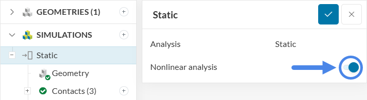
A nonlinear static analysis makes it possible to account for effects such as:
- Non-elastic material behavior (plasticity in this case)
- Large displacements and rotations
This approach ignores inertia effects. This differs from a Dynamic analysis, which accounts for inertial forces.
2. Set Up the Simulation
This tutorial simulates the forming process of an aluminium pipe using a hydraulic bending machine and evaluates the mechanical stress and strain induced in the part(s). The image below illustrates the model components and the process:
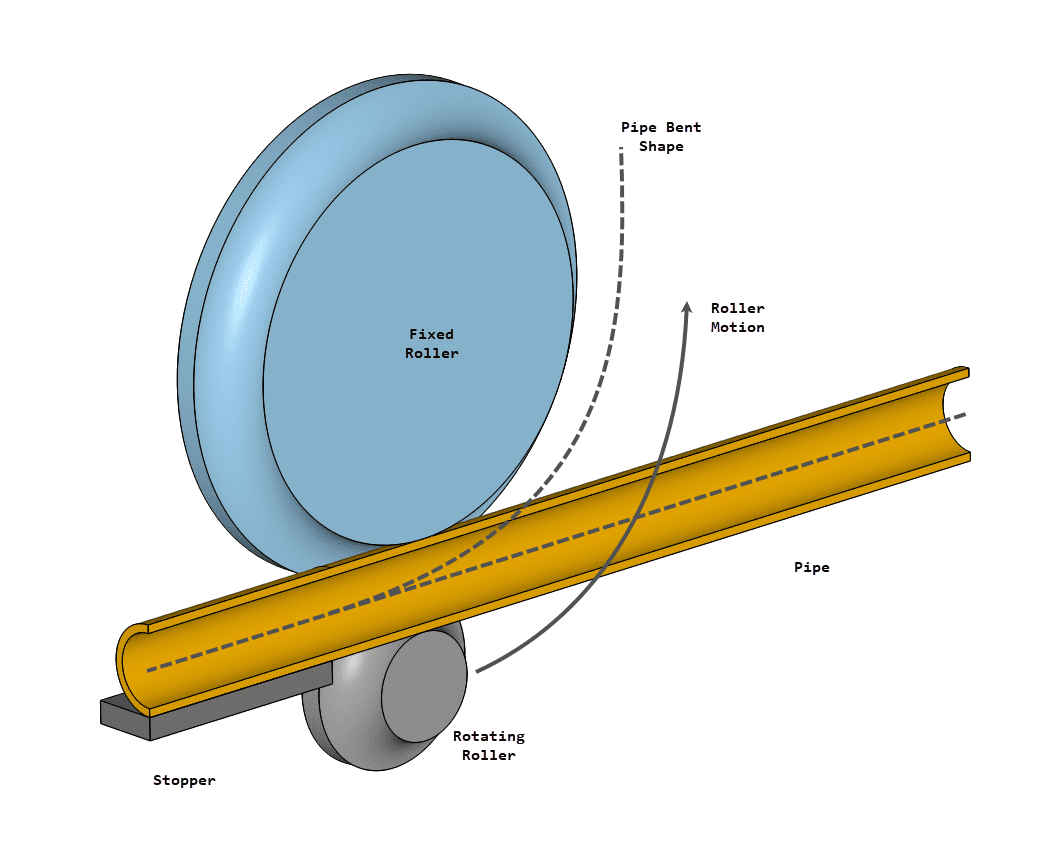
The following modeling techniques are used to simulate the process:
- The pipe deformation requires an Elasto-plastic material model.
- The contact areas between the pipe and the rollers change during the simulation, and contact forces drive the deformation, so these interfaces are modeled as Physical contact.
- A Bonded contact is used between the pipe and the stopper to prevent movement at one pipe end.
- As shown in Figure 6, the rotating roller bends the pipe around the fixed roller, so a Rotating motion is assigned to the small roller using the large roller as the center.
- Because the geometry and boundary conditions are symmetric, only half of the model is simulated and a symmetry condition is applied, reducing computational cost.
2.1. Contacts
With the analysis type selected, some contacts are detected automatically:
- Between the small roller and the pipe
- Between the large roller and the pipe
- Between the pipe and the stopper
Only the contact between the pipe and the stopper will be kept — although altered — since there should be no relative motion between their contact nodes. The other two contact relationships are modeled using Physical Contacts instead, which captures real interactions between components, such as coming in and out of contact.
Refer to this documentation page for more information about contacts.
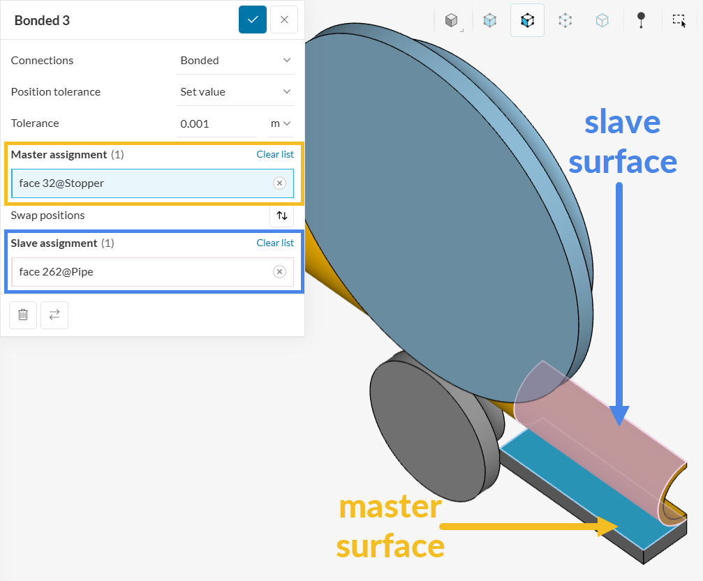
A. Bonded Contact
SimScale automatically detects touching faces or edges in the geometry and assigns bonded contacts by default. In this case, the three contacts listed above are detected:
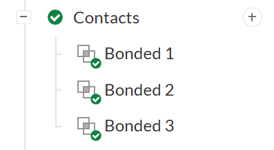
A bonded contact is only required between the pipe and the stopper (Bonded 3), so the other two contacts must be deleted manually:
- On the Contacts node, right-click the contact interaction to be deleted (for example, Bonded 1)
- Click Delete
- Repeat the process for the other contact (Bonded 2 in this case)
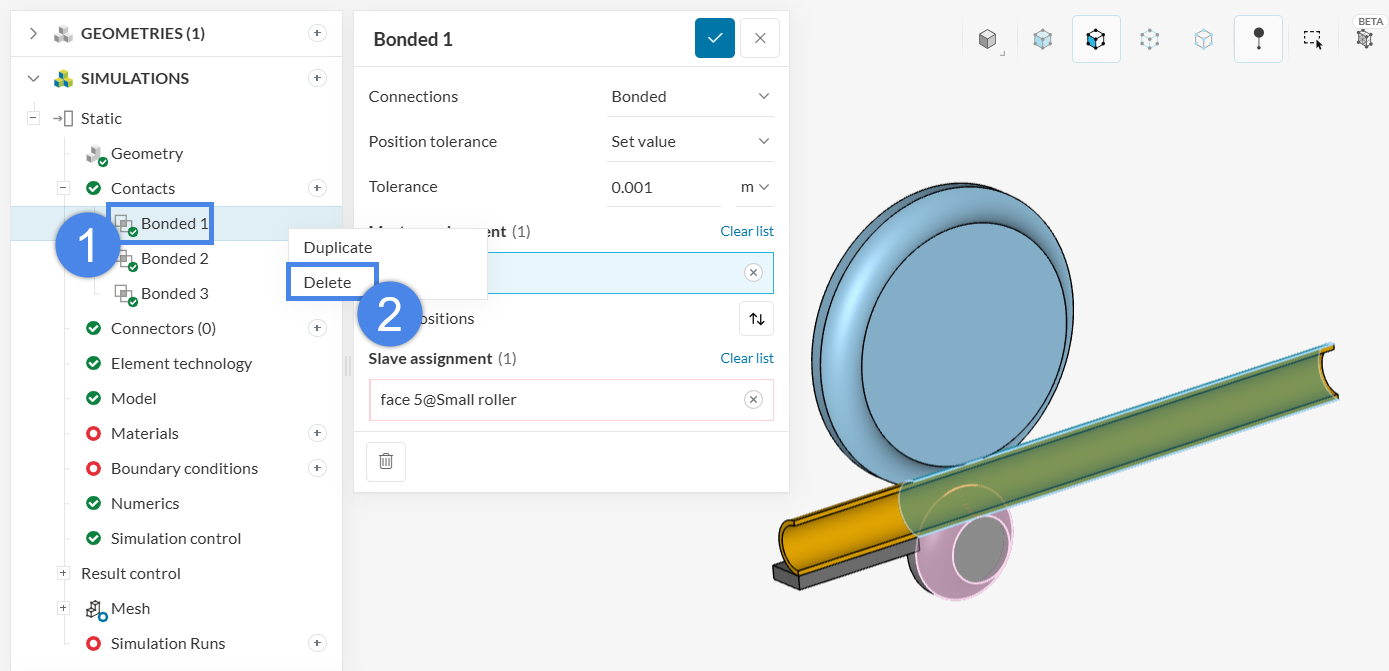
For Bonded 3, ensure the correct faces are assigned to the Master and Slave assignments, namely, the bottom face of the stopper and the pipe’s face in contact with it:
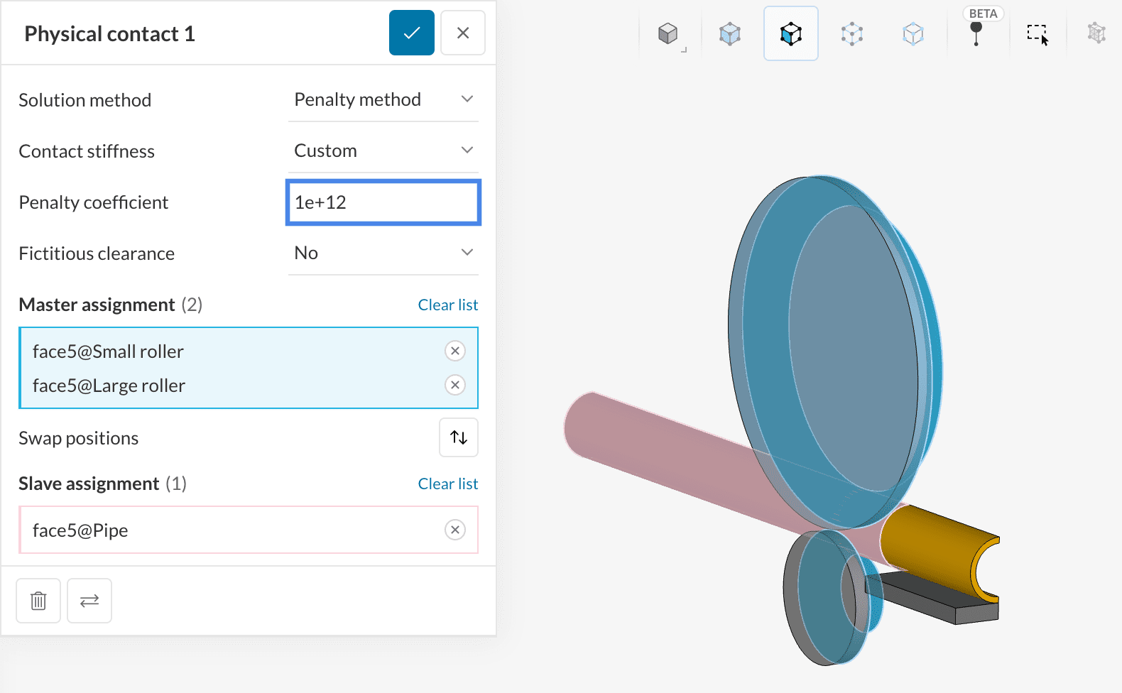
B. Physical Contacts
Next, assign Physical Contacts. Physical contacts are used for interfaces where surfaces can slip, come into contact, separate, and transfer forces during the simulation, such as between the pipe and the rollers. Friction can also be included, but it is not required in this case. Follow the steps below to create the physical contact model:
- Click the + icon next to Physical Contacts.
- Set the Penalty Coefficient to 1e+12 by selecting a Custom contact stiffness.
- Assign the faces as shown in the image:
Note
If you are not sure which surface to choose as the master and which as the slave in your own simulation, refer to this knowledge base article.
2.2. Model & Element Technology
Leave both panels at their default settings, and proceed to Materials.
2.3. Assign Materials
Two different materials are used for this simulation:
- Steel for the rollers and stopper. This material is linear elastic, as these bodies remain rigid.
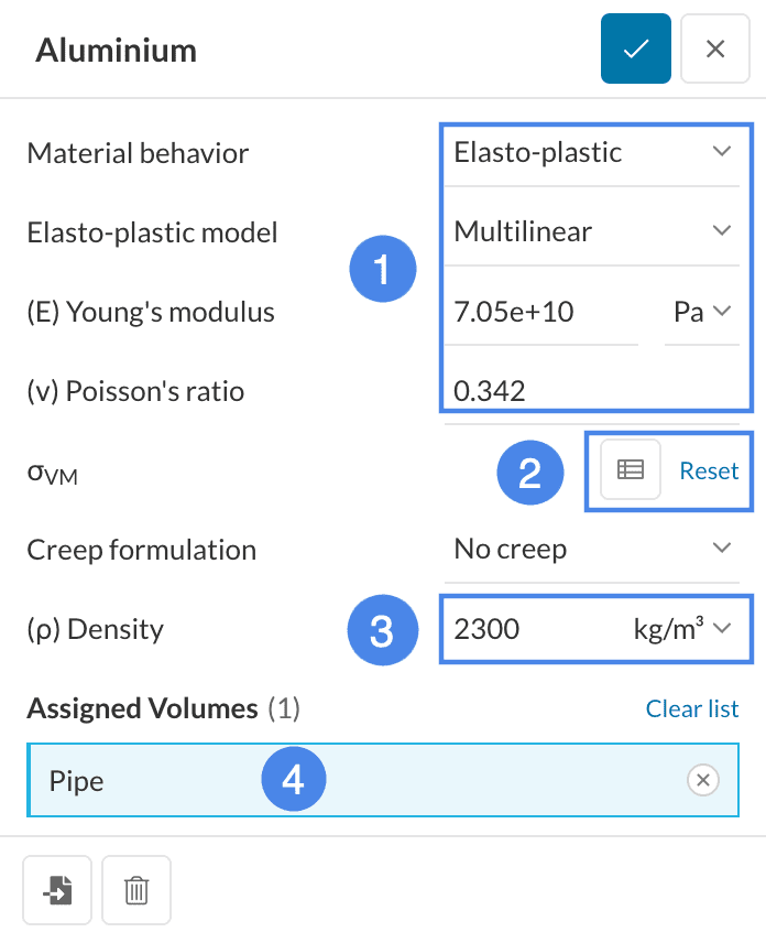
- Aluminium for the pipe. This material uses an Elasto-plastic model, as it undergoes large deformations.
To create a new material, click the + icon next to Materials. The materials library opens. Select the desired material from the list and click Apply to create the material item, as shown in the image:
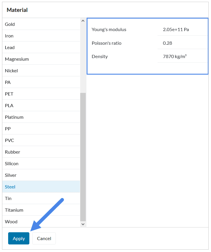
First, create a Steel material item and assign it to the Stopper, Small roller, and Large roller bodies. All other parameters can remain at their default values:

For the pipe, create an Aluminium material using the same procedure. Notice that the pipe body is automatically selected, as it is the only one without a material assignment.
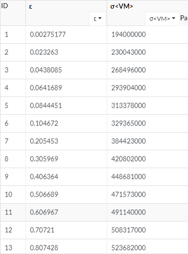
The image below shows the true stress-strain curve for the material, including its elasto-plastic behavior. Switching the material behavior to elasto-plastic enables permanent deformation, whereas an elastic model causes the body to return to its original shape after unloading.
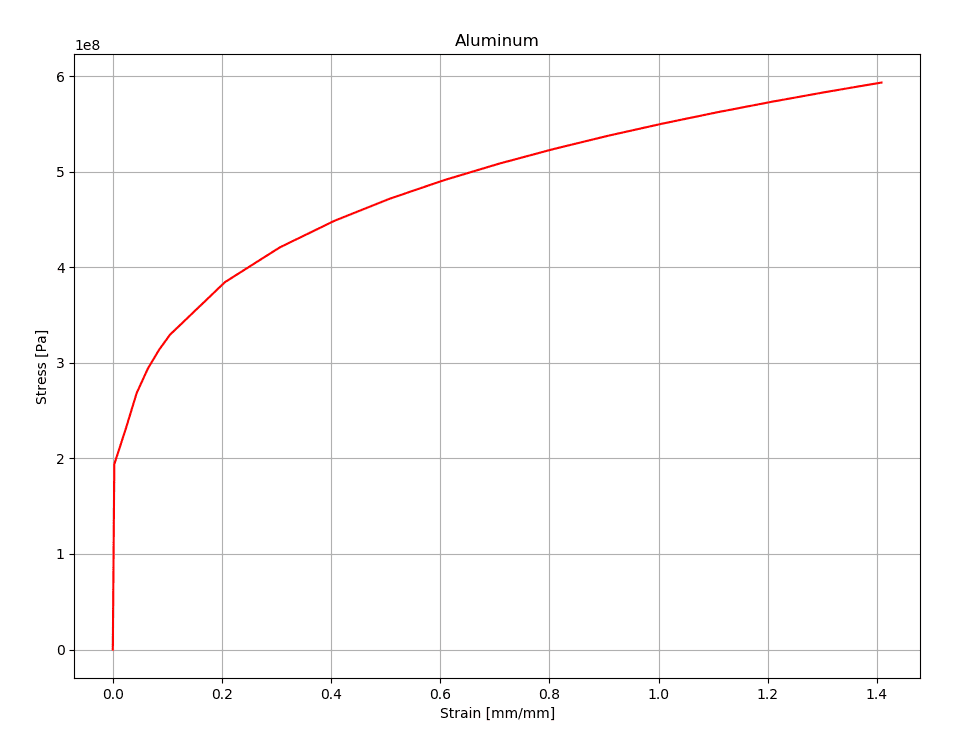
To model this nonlinear behavior, change the Material behavior to Elasto-plastic and set the other parameters as shown. Note that the stress curve \(\sigma\)<VM> data is missing and will be provided in the next steps.
The solver requires the aluminium stress-strain curve shown in Figure 13 to predict deformation. This curve is provided as a table. Use the button below to download the material data as a CSV file:
Plastic Curve Data
If you examine or plot the CSV table, you will notice that it only includes the plastic part of the curve. That is, the [0,0] point is not in the curve, and it starts at the yield point. This convention should always be followed when uploading plastic curve data.
Now click the table input button in the material window (highlighted in Step 2 from Figure 13). This opens the Specify value window:
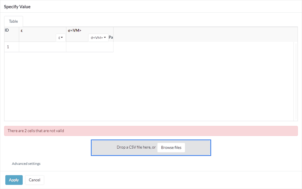
Click the Browse files button to select and upload the previously downloaded CSV file. The \(\varepsilon – \sigma\) table should populate with the data as follows:
After uploading the table, click Apply in the settings shown in Figure 14 to confirm the data, then click the check-mark button in the material window (Figure 14) to save the setup. The error message shown in Figure 15 should now be resolved.
2.4. Initial and Boundary Conditions
For this simulation, the initial conditions can be left unchanged.
Review Figure 7 for an overview of the physical setup and to better understand the boundary conditions defined in this section.
To create a boundary condition, click the + button next to Boundary conditions in the left panel, then select the required boundary condition type from the drop-down menu, as shown in the figure:
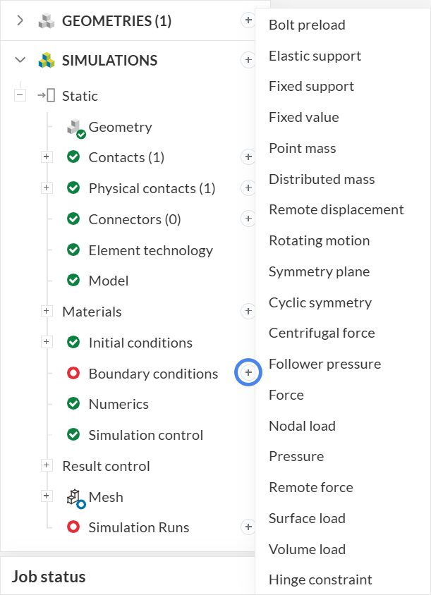
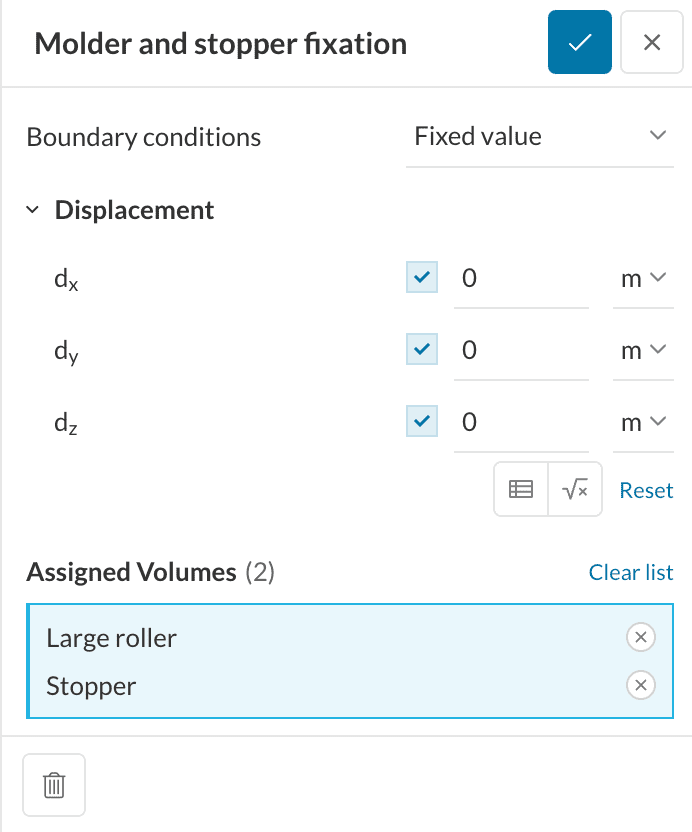
A. Fixed Roller and Stopper
Create a Fixed value boundary condition.
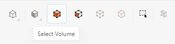
By default, Face selection mode is active. To assign a solid body, use the scene tree on the right side of the workbench to switch to volume selection mode:
Assign the boundary condition to the Large roller and Stopper bodies. Both must be prevented from moving, as shown in Figure 6, so the displacement in X, Y and Z must be constrained (set to 0).
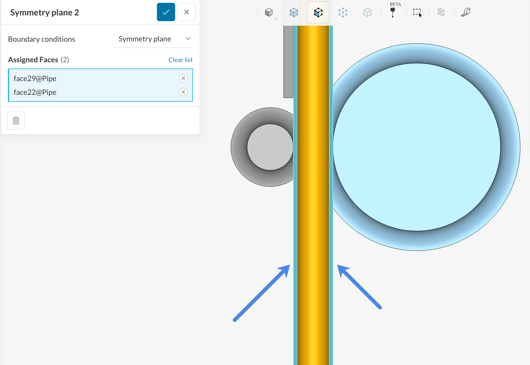
B. Pipe Symmetry Plane
The geometry includes only half of the pipe and the other bodies, which reduces mesh size and computational cost. Apply a Symmetry plane boundary condition to the flat faces of the pipe (the other bodies are constrained through other boundary conditions, so they are not included here). Create the boundary condition as described above and assign the pipe symmetry faces as shown in the image:
C. Moving Roller Rotation
For the motion of the small roller, use a Rotating motion boundary condition.
In this model, the rotation axis passes through the origin and is oriented in the X-direction. For other models, obtain the axis position and orientation from CAD and enter them in the boundary condition. Create the Rotating motion and assign the top face of the Small roller. Set up the parameters as shown:
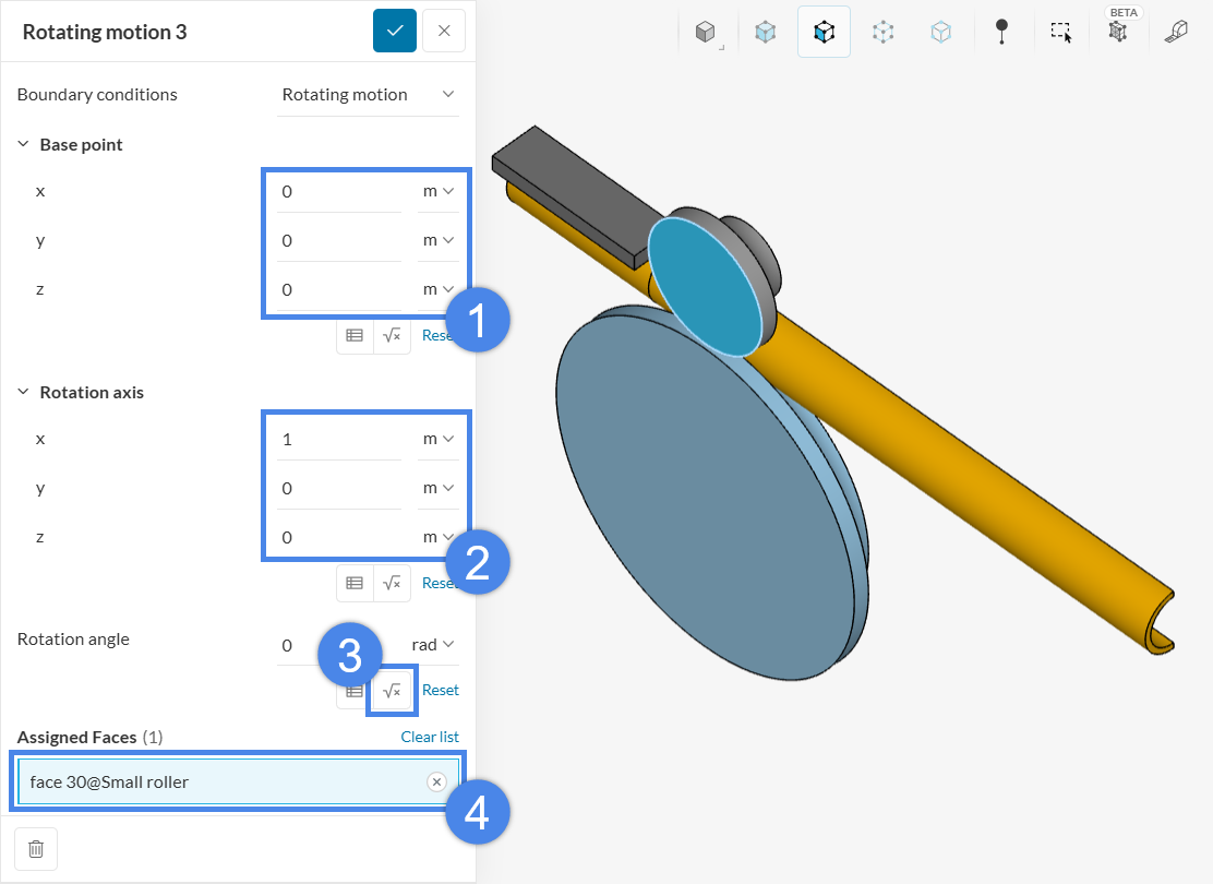
To specify the rotation angle, use an equation input. The angle should increase linearly from zero to the maximum value over the simulated time. The image below illustrates the simulated motion:
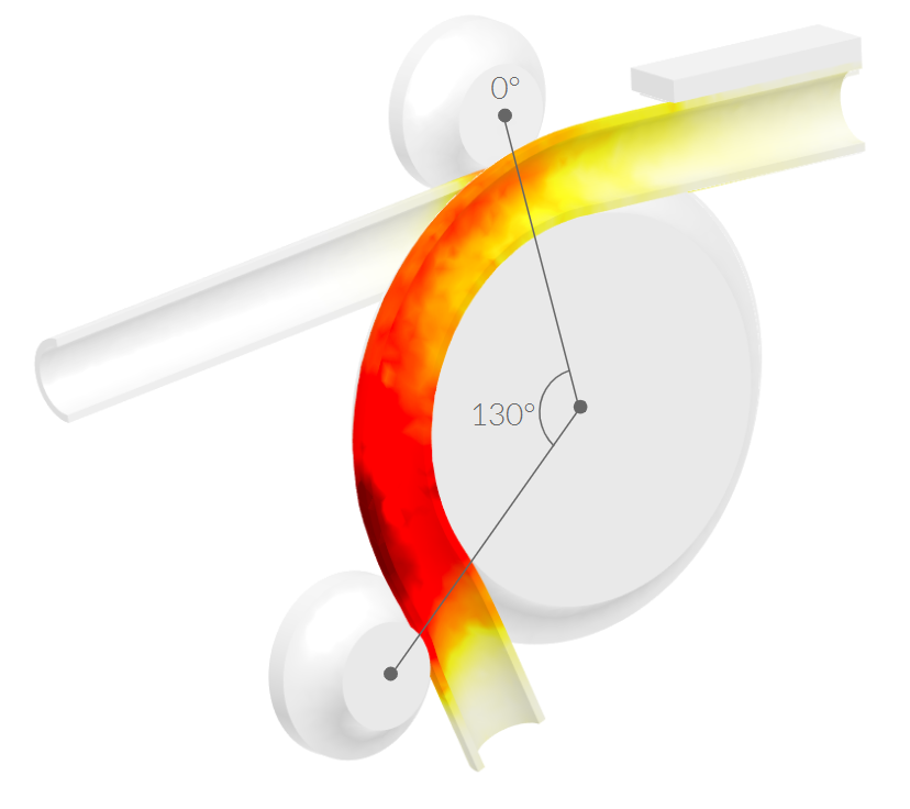
Account for the right-hand rule and the specified rotation axis direction to obtain the correct rotation direction. In this case, a positive 130° roller rotation is required to achieve the target pipe bending angle. The corresponding equation is:
$$\phi(t) = 130 \times t$$
To add the equation, click the formula button in the rotating motion boundary condition window (highlighted in Step 3 in Figure 21).
The Specify value window appears. Enter the formula as shown in Figure 23 and change the unit from rad to º.
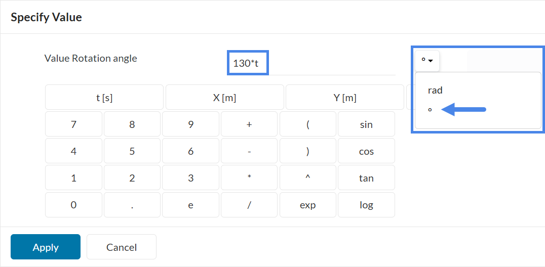
Click the Apply button (in Figure 23) and the ‘check-mark’ button (in Figure 21) to save the setup.
2.5. Numerics and Simulation Control
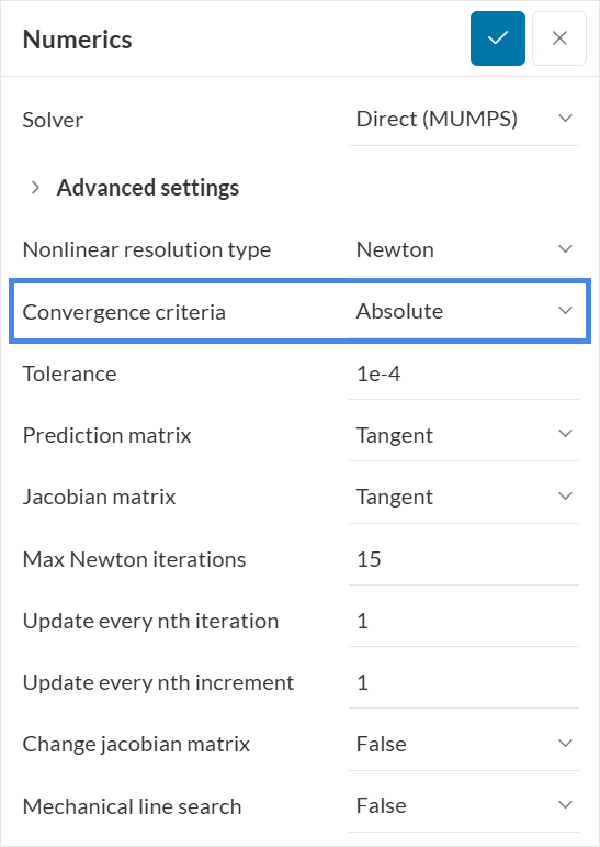
The Numerics parameters control solver behavior and precision. In this case, only one parameter needs to be changed: Convergence criteria. The default Relative criteria use the applied load magnitude to check convergence. That approach does not work here because the model is driven by an imposed displacement, so no loads are defined. Change the criteria to Absolute, as shown in the image:
The Simulation control parameters define the simulation time, time step, time adaptation, and output write interval. Set the simulation control values as shown below:
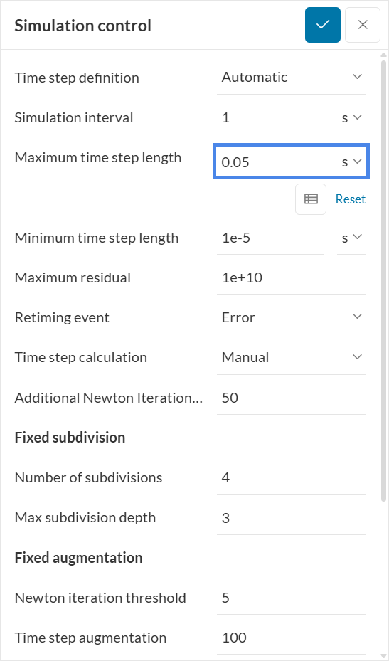
Leave the Simulation interval at the default value of 1 \(s\). This means the simulation runs from 0 to 1 \(s\), matching the interval used to define the roller rotation. Set the Maximum time step length to 0.05 \(s\) to obtain 20 integration steps in the [0,1] \(s\) interval.
2.6. Result Control
Result control defines which result fields are written during the simulation, such as displacements, strains, and stresses, along with characteristics such as average or maximum values. Several default fields are provided, but additional fields are required for this case:
A. Solution Fields
Two additional result fields will be queried from the solver:
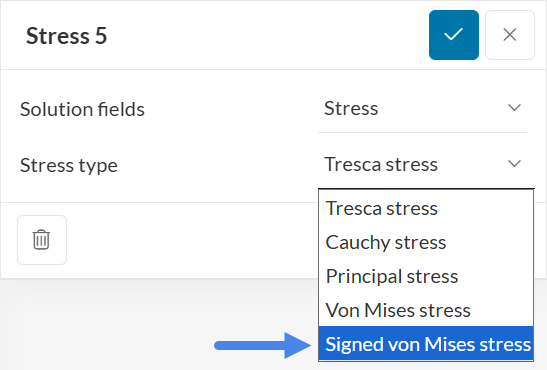
- Signed von Mises stress: used to assess failure according to distortion energy theory, while distinguishing regions in tension (positive stress) and compression (negative stress).
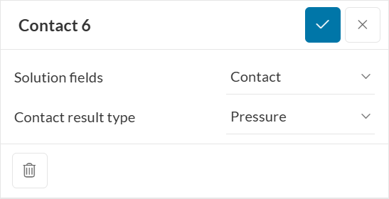
- Contact pressure: used to evaluate transferred forces through a contact interface as a distributed pressure field.
To create the additional solution fields:
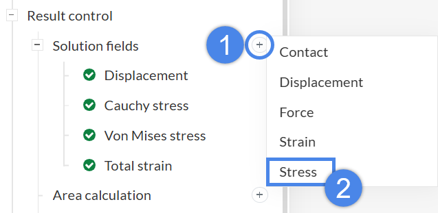
- Click the + icon next to Solution fields, under Result control
- Select the field type from the drop-down menu.
First, create a Stress field and change the stress type to Signed von Mises stress.
Then, create a Contact field and keep the default parameters:
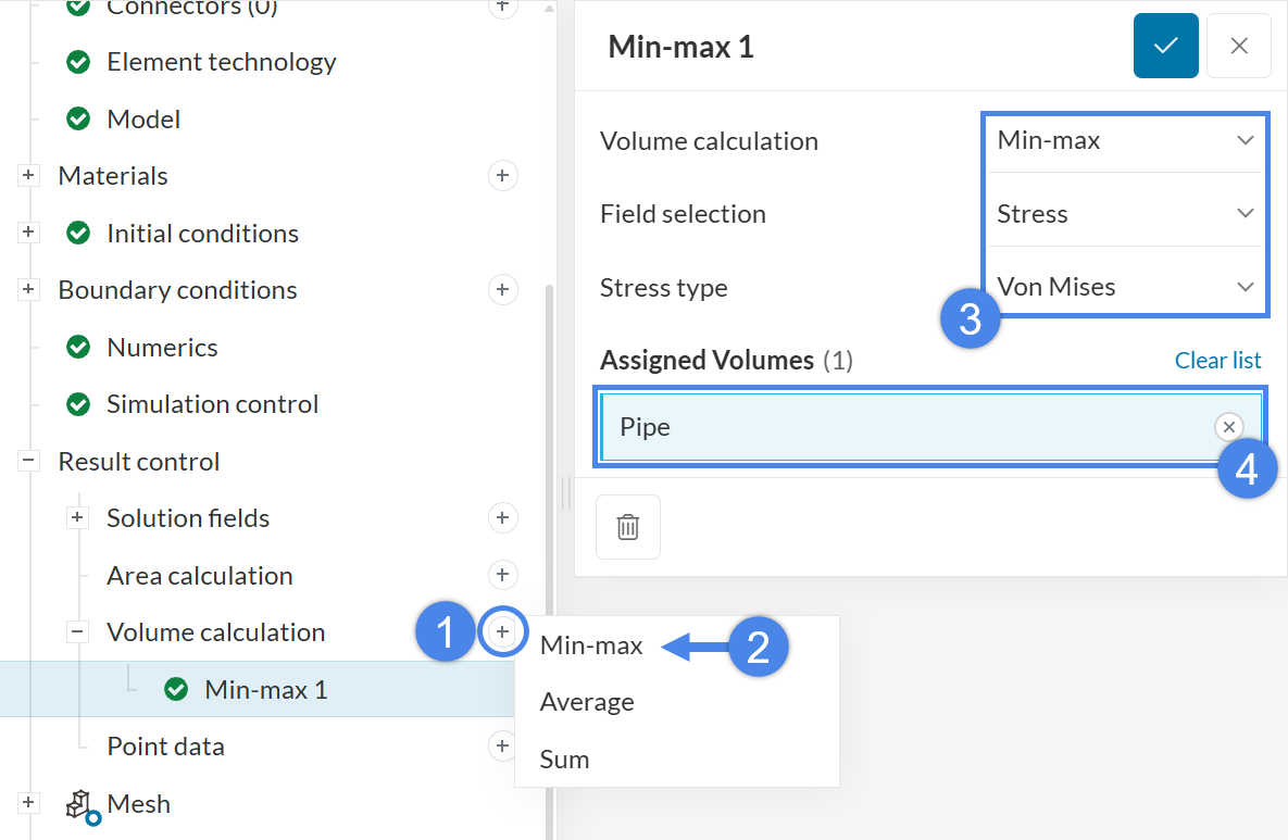
B. Volume Calculation
Volume calculations compute statistics of a field over a part and report them as curves over the simulation interval. In this case, two volume calculations will be added:
- Minimum and maximum values of the von Mises stress, to identify the lowest and highest stress levels in the pipe.
- Minimum and maximum values of the signed von Mises stress, to identify peak compression and tension stresses in the pipe.
To add a volume calculation, follow these steps:
- Click the ‘+’ icon next to Volume calculation under Result control
- Select the statistic type from the drop-down list.
Use the steps above to create a Volume calculation – Min-max item and set it up for the von Mises stress field over the pipe, as shown in the image:
- Change the Field selection to Stress.
- Select the Von Mises Stress type.
- Assign this calculation to the Pipe. Select it by clicking in the viewer.
Repeat the same steps to create the Signed von Mises Stress min-max item.
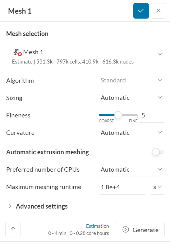
3. Mesh
The standard mesh algorithm will be used. In this case, the general settings can remain at their default values:
Mesh refinements allow control of the local element size on selected faces and volumes. They are primarily used to optimize computational resources: instead of increasing fineness globally, apply refinements locally to limit the impact on cell count. In addition, Extrusion mesh refinements can be used to improve the mesh in thin sections, which can otherwise cause distortions in non-organized meshes.
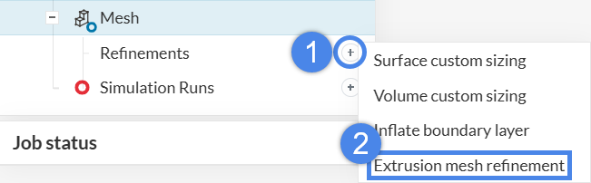
- Click the + icon next to Refinements under Mesh
- Select the refinement type from the drop-down list.
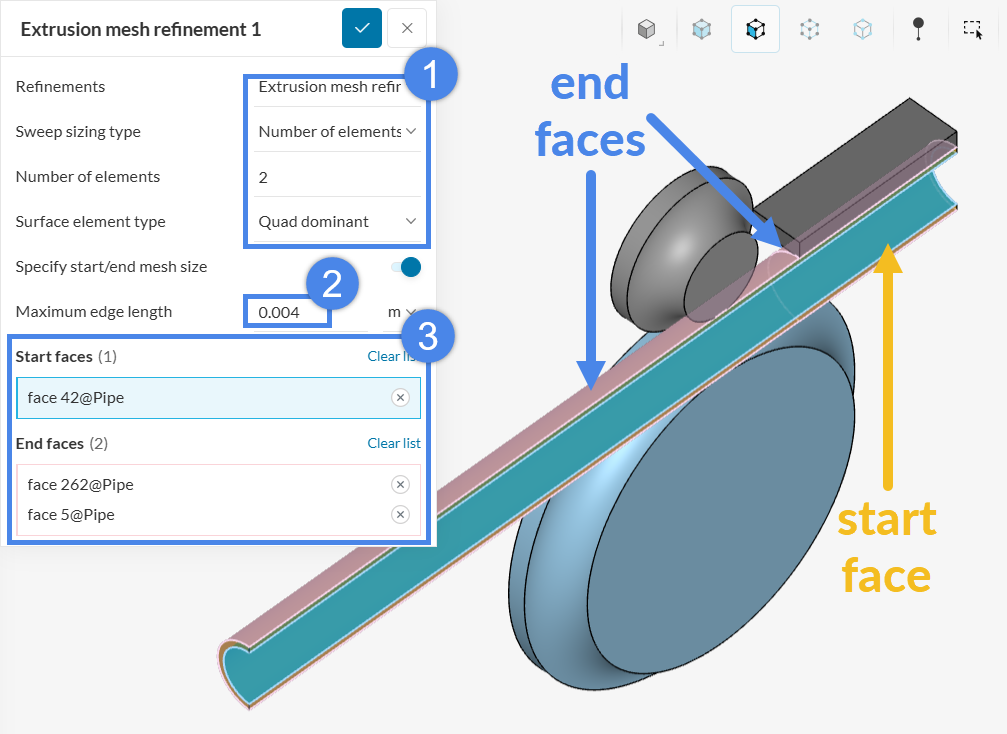
Apply an Extrusion mesh refinement to the indicated faces of the pipe (Figure 31). The mesh is generated on the start face and then extruded through the thickness direction to the end faces (note that the outer face is split in two). After selecting the start and end faces, set the Sweep sizing type to Number of elements along sweep, set the value to 2, and set the Surface element type to Quad dominant. To increase surface fineness, enable Specify start/end mesh size and set a Maximum edge length of 4e-3m.
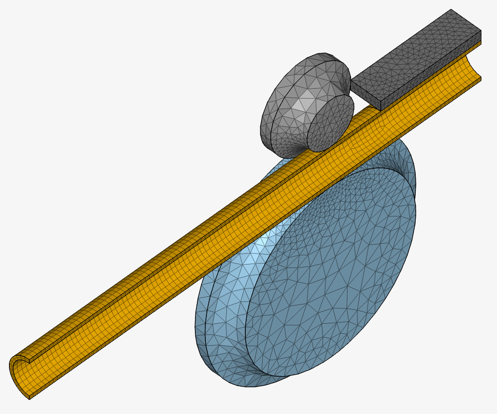
There is no need to generate the mesh at this point, as it will be computed as part of the simulation run. When mesh computation is complete, it will be marked with a green check-mark icon. The mesh can then be opened to review the final result:
4. Start the Simulation
Create a new run by clicking the + icon next to Simulation Runs in the tree, as shown below:
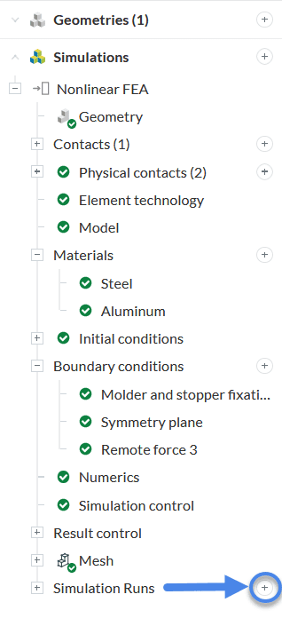
In the pop-up dialog, name the run and start the simulation. Once it completes, the results can be reviewed.
Important
When you create a simulation run, the following warning message will appear:
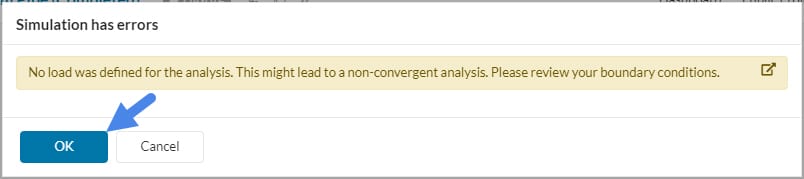
For this tutorial, the run will be successful, so the warning message can be ignored by clicking the ‘OK’ button.
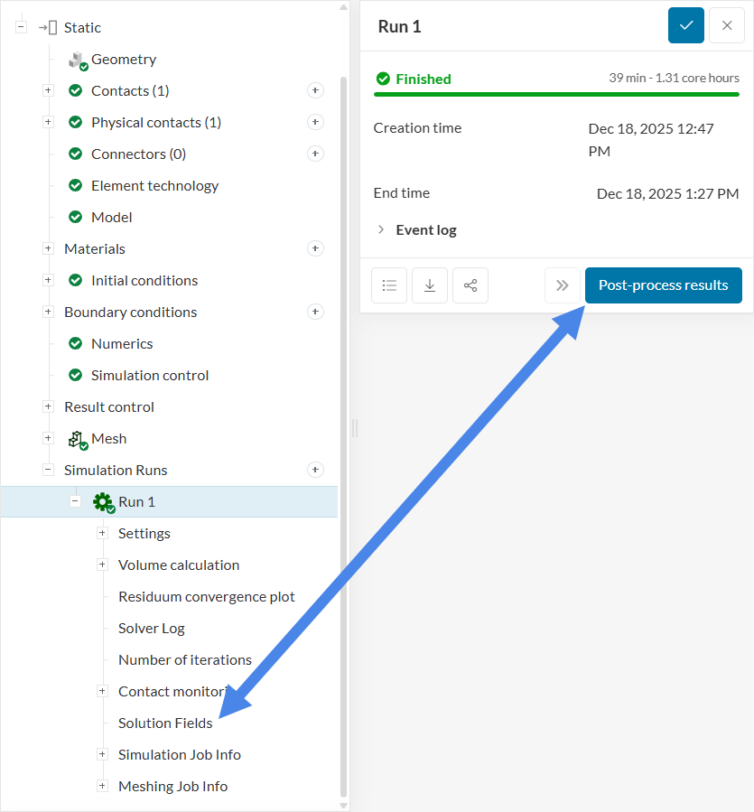
5. Post-Processing
After the simulation run finishes, the pipe bending results can be post-processed. The online post-processor can be opened in one of two ways:
- Click Solution Fields under the completed run.
- Click the Post-process results button in the run dialog.
5.1 Deformations
After the solution fields load, Von Mises Stress is selected by default as Coloring under Parts Color and is plotted on the deformed shape using Displacement for the last time step. Right-click the legend bar and select Use Continuous Scale to display a smoother result visualization.
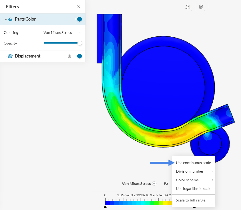
The following plot is displayed:
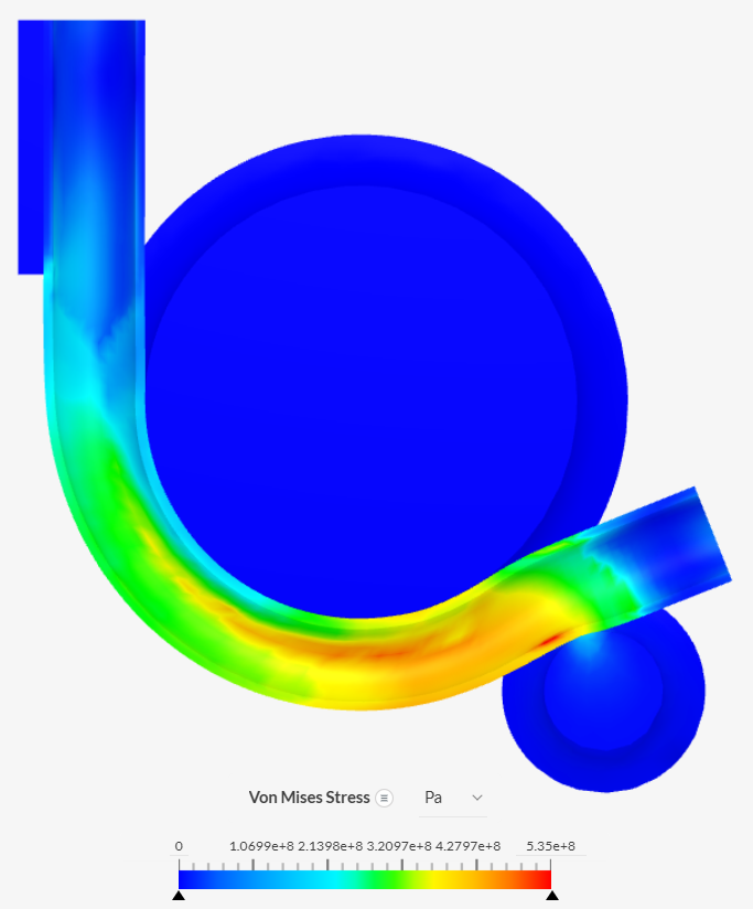
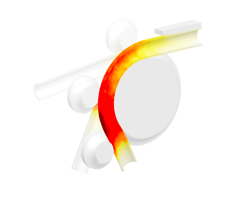
The pipe follows the rig geometry, and the bending behavior is captured successfully.
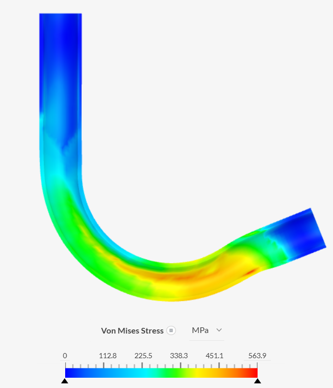
5.2 Stress
To make the legend scale easier to interpret, apply the following changes while the Von Mises Stress field is visible:
- Change the stress units to \(MPa\).
- Set the maximum scale value to the yield stress of 194 \(MPa\).
- Rotate the model to visualize the internal section of the pipe.
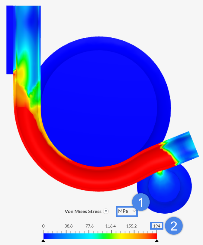
Regions of the pipe that exceed the yield point are shown in red. The Hertzian contact stress on the follower body can also be observed.
5.3 Animation
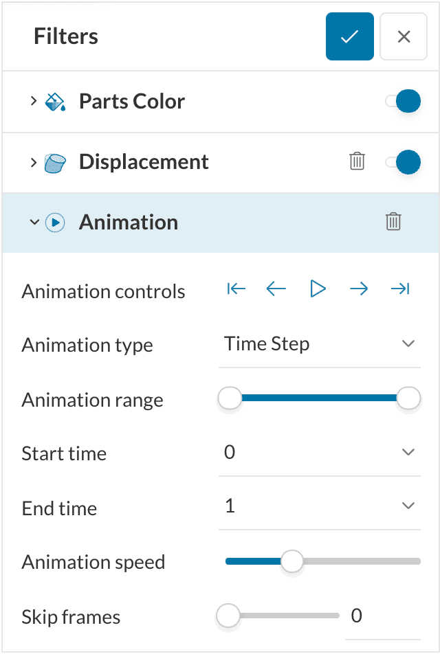
The bending process can also be visualized as an animation. To create it, add an Animation filter the same way the Displacement filter was created:
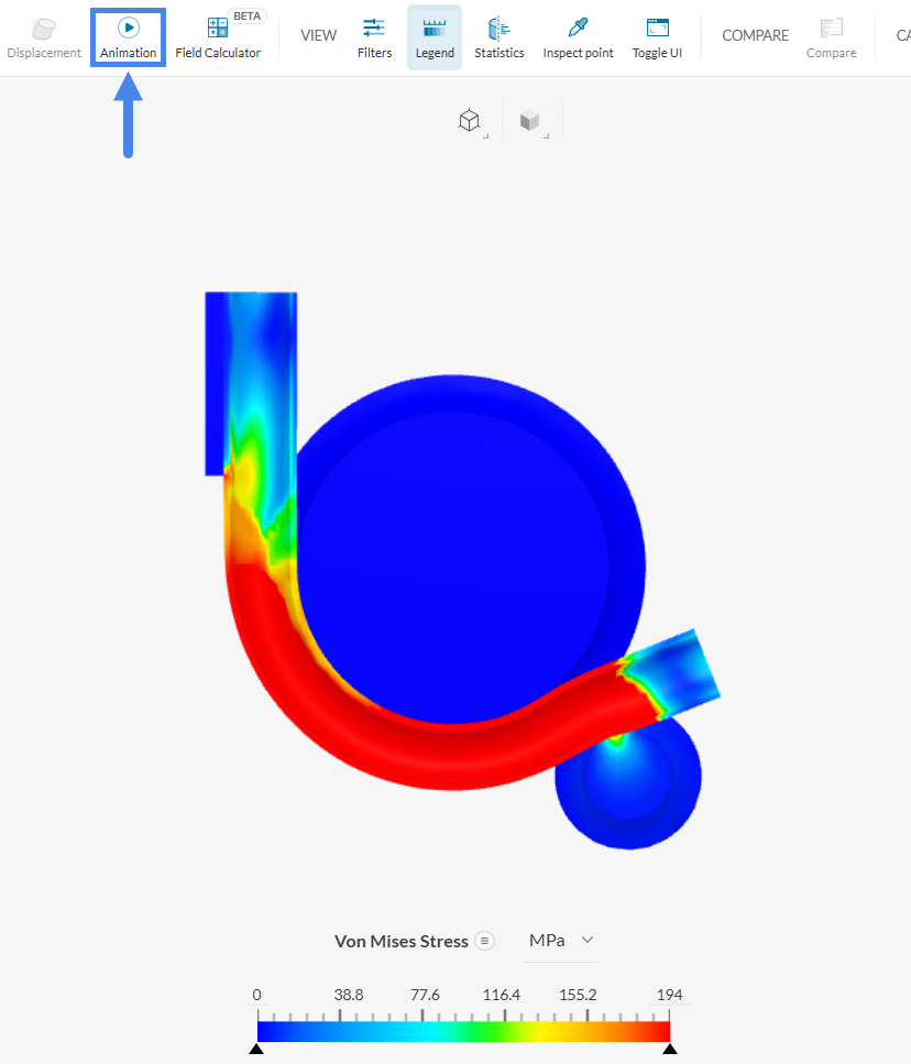
The default filter parameters are sufficient for this purpose:
Click Play under Animation controls to start the bending animation:
5.4 Part Visibility
To better visualize stress in the bent pipe, hide all other parts as follows:
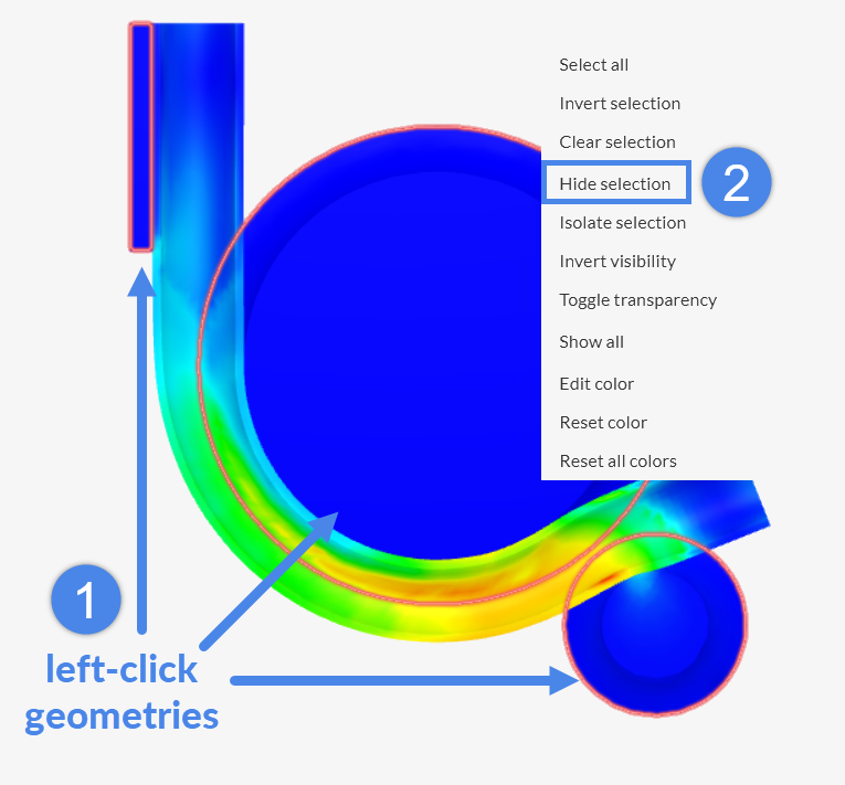
- Left-click to select all parts except the pipe
- Right-click to open the context menu
- Select Hide Selection
The stress distribution on the bent pipe can now be inspected without other parts obstructing the view. Higher stress levels occur on the outer portion of the pipe, close to the contact region with the roller.
Explore how each parameter affects the results and try different visualizations. For more details on SimScale’s online post-processor, refer to the post-processing guide.
Congratulations! The tutorial is complete.
Note
If you have any questions or suggestions, please reach out via the forum or contact us directly.
Last updated: December 23rd, 2025
Did this article solve your issue?
How can we do better?
We appreciate and value your feedback.


