Documentation
The dimensionless Reynolds number plays a prominent role in foreseeing the patterns in a fluid’s behavior. The Reynolds number, referred to as Re, is used to determine whether the fluid flow is laminar or turbulent. Along with the Nusselt number for heat transfer and the Prandtl number for fluid properties, it is one of the main controlling parameters in all viscous flows where a numerical model is selected according to a pre-calculated Reynolds number.
Although the Reynolds number comprises both static and kinetic properties of fluids, it is specified as a flow property since dynamic conditions are investigated. Technically speaking, the Reynolds number is the ratio of the inertial forces to the viscous forces. This ratio helps to categorize laminar flows from turbulent ones.
Inertial forces resist a change in the velocity of an object and are the cause of fluid movement. These forces are dominant in turbulent flows. Otherwise, if the viscous forces, defined as the resistance to flow, are dominant – the flow is laminar. The Reynolds number can be specified as below:
$$ Re=\frac{inertial~force}{viscous~force}=\frac{fluid~and~flow~properties}{fluid~properties} \tag{1}$$
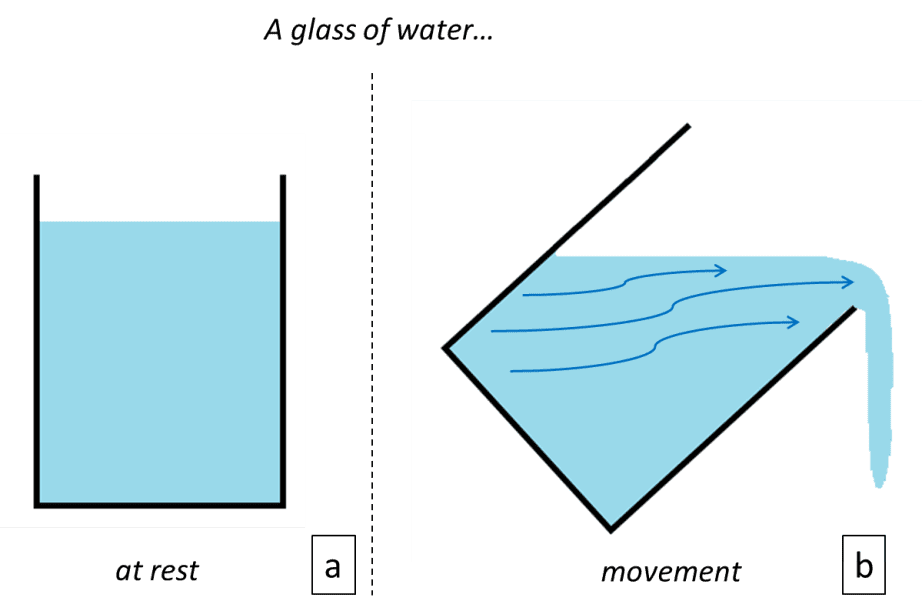
For instance, a glass of water that stands on a static surface, regardless of any forces apart from gravity, is at rest, and flow properties are ignored. Thus, the numerator in equation (1) is “0”. That results in independence from the Re for a fluid at rest. On the other hand, whilst water is spilled by tilting a water-filled glass a Reynolds number can be estimated to predict fluid flow that is illustrated in Figure 1.
The theory of a dimensionless number that predicts fluid flow was initially introduced by Sir George Stokes (1819-1903) who had attempted to figure out drag force on a sphere whereby neglecting the inertial term. Stokes had also carried out the studies of Claude Louis Navier (1785-1836) taking them further and deriving the equation of motion by adding a viscous term in 1851 – thereby revealing the Navier-Stokes equation\(^1\).
Stokes flow, named after Stokes’ approach to viscous fluid flow, is the mathematical model in which the Re is so low that it is presumed to be zero. Various scientists had conducted studies to examine the properties of fluid movement after Stokes. Even though the Navier-Stokes equations thoroughly analyzed fluid flow, it was quite hard to apply them to arbitrary flows where the Reynolds number could easily predict fluid movement.
In 1883, Irish scientist Osborne Reynolds discovered the dimensionless number that predicts fluid flow based on static and dynamic properties such as velocity, density, dynamic viscosity and characteristics of the fluid\(^2\). He conducted experimental studies to examine the relationship between the velocity and behavior of the fluid flow. For this purpose, an experimental setup (Figure 2a) was established by Reynolds using dyed water which was released in the middle of the cross-sectional area into the main clear water to visualize the movement of fluid flow through the glass tube (Figure 2b).

The study of Osborne Reynolds titled ‘An experimental investigation of the circumstances which determine whether the motion of water in parallel channels shall be direct or sinuous’ regarding the dimensionless number was issued in “Philosophical Transactions of the Royal Society”. According to the article, the dimensionless number discovered by Reynolds was suitable to foresee fluid flow in a broad range from water flow in a pipe to airflow over an airfoil\(^2\).
The dimensionless number was referred to as parameter :math:‘R’, until the presentation of German physicist Arnold Sommerfeld (1868 – 1951) at the 4th International Congress of Mathematicians in Rome (1908), where he referred to the ‘R’ number as the ‘Reynolds number’. The term used by Sommerfeld has been used worldwide ever since\(^3\).
The dimensionless Reynolds number predicts whether the fluid flow would be laminar or turbulent referring to several properties such as velocity, length, viscosity, and also type of flow. It is expressed as the ratio of inertial forces to viscous forces and can be explained in terms of units and parameters respectively, as below:
$$ Re=\frac{ρVL}{μ}=\frac{VL}{v} \tag{2}$$
$$ Re=\frac{F_{inertia}}{F_{viscous}}=\frac{\frac{kg}{m^3}\times{\frac{m}{s}}\times{m}}{Pa\times{s}}=\frac{F}{F} \tag{3}$$
where \(ρ~(\frac{kg}{m^3})\) is the density of the fluid, \(V~(\frac{m}{s})\) is the characteristic velocity of the flow, and \(L~(m)\) is the characteristic length scale of flow. Equation (3) is the derivation of units at which the Re is specified as non-dimensional. Variations of the Reynolds number are shown in equation (2) where \(μ (Pa\times{s})\) is the dynamic viscosity of fluid and \(v~(\frac{m^2}{s})\) is the kinematic viscosity. The transition between dynamic and kinematic viscosity is as follows:
$$ v=\frac{μ}{ρ} \tag{4}$$
The applicability of the Reynolds number differs depending on the specifications of the fluid flow such as the variation of density (compressibility), variation of viscosity (Non-Newtonian), internal or external flow, etc. The critical Reynolds number is the expression of the value to specify transition among regimes which diversifies regarding the type of flow and geometry as well.
Whilst the critical Reynolds number for turbulent flow in a pipe is 2000, the critical Reynolds number for turbulent flow over a flat plate, when the flow velocity is the free-stream velocity, is in a range from \(10^5\) to \(10^6\). \(^4\)
The Reynolds number also predicts the viscous behavior of the flow in case fluids are Newtonian. Therefore, it is highly important to perceive the physical case to avoid inaccurate predictions. Transition regimes and internal & external flows are the basic fields to comprehensively investigate the Reynolds number.
Newtonian fluids are fluids that have a constant viscosity. If the temperature stays the same, it does not matter how much stress is applied on a Newtonian fluid; it will always have the same viscosity. Examples include water, alcohol and mineral oil.
The fluid flow can be specified under two different regimes: Laminar and Turbulent. The transition among the regimes is an important issue that is driven by both fluid and flow properties. As mentioned before, the critical Reynolds number can be classified as internal and external. Yet while the Reynolds number regarding the laminar-turbulent transition can be defined reasonably for internal flow, it is hard to specify a definition for external flow.
The fluid flow in a pipe as an internal flow had been illustrated by Reynolds as in Figure 2b. The critical Reynolds number for internal flow is: \(4\)
| Flow type | Reynolds Number Range |
|---|---|
| Laminar regime | up to Re=2300 |
| Transition regime | 2300<Re<4000 |
| Turbulent regime | Re>4000 |
Open-channel flow, fluid flow in an object, and flow with pipe friction are internal flows in which the Reynolds number is predicted based on hydraulic diameter \(D\) instead of characteristic length \(L\). In case the pipe is cylindrical, the hydraulic diameter \(D\) is accepted as the actual diameter of the cylinder, meaning the Reynolds number is as follows:
$$ Re=\frac{F_{inertia}}{F_{viscous}}=\frac{ρVD_H}{μ} \tag{5}$$
The shape of a pipe or duct can vary (e.g. square, rectangular, etc.). In those cases, the hydraulic diameter is determined as below:
$$ D_H=\frac{4A}{P} \tag{6}$$
where \(A\) is the cross-sectional area and \(P\) is the wetted perimeter.
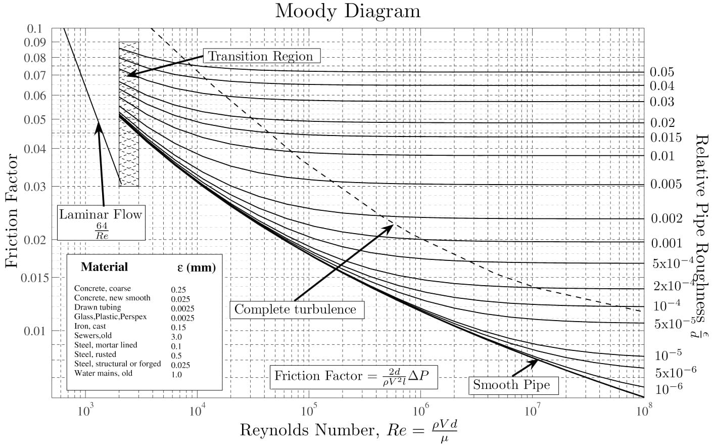
The friction on the pipe surface due to roughness is an effective parameter to consider because it causes laminar to turbulence transition and energy losses. The ‘Moody Chart’ (Figure 4) was generated by Lewis Ferry Moody (1944) to predict fluid flow in pipes where roughness was effective. It is a practical method to determine energy losses in terms of friction factor due to roughness throughout the inner surface of a pipe. The critical Reynolds number for a pipe with surface roughness abides by the regimes above\(^2\).
In the chart below you can see a logarithmic scale at the bottom with a scale for the friction factor at the left and the relative roughness of the pipe at the right.
External flow at which mainstream has no distinct boundaries is alike to internal flow that also has a transition regime. Flows over bodies such as a flat plate, cylinder and sphere are the standard cases used to investigate the effect of velocity throughout the stream. In 1914, German scientist Ludwig Prandtl discovered the boundary layer, which is partially the function of the Reynolds number, covering the surface through laminar, turbulent and also transition regimes \(^5\). The flow over a flat surface is shown in Figure 5 with regimes where \(x_c\) is the critical length for transition, \(L\) is the total length of the plate and \(u\) is the velocity of the free streamflow.
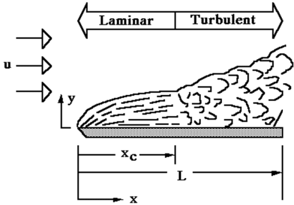
In general, the boundary layer dilates with movement through \(x\) direction on plate that eventually results in unstable conditions where the Reynolds number increases simultaneously. The critical Reynolds number for flow over flat plate surface is:
$$ Re_{critical}=\frac{ρVx}{μ}≥3\times{10^5}~to~3\times{10^6} \tag{7}$$
which depends on the uniformity of the flow over the surface. Yet while the critical Reynolds numbers for regimes are virtually specified for internal flow, it is hard to detect them for an external flow which diversifies the critical Reynolds number regarding geometry. Furthermore, apart from internal flow, boundary layer separation is an anomalous issue for external flow where several ambiguities are encountered to generate a reliable numerical model with respect to a physical domain.\(^6\)
Reynolds number is also effective on Navier-Stokes equations to truncate mathematical models. While \(Re→∞\), the viscous effects are presumed negligible where viscous terms in Navier-Stokes equations are dropped. The simplified form of the Navier-Stokes equations — called Euler equations — can be then specified as follows:
$$ \frac{Dρ}{Dt}=-ρ∇\times{u} \tag{8}$$
$$ \frac{Du}{Dt}=-\frac{∇p}{ρ}+g \tag{9}$$
$$ \frac{De}{Dt}=-\frac{p}{ρ}∇\times{u} \tag{10}$$
where \(ρ\) is density, \(u\) is velocity, \(p\) is pressure, \(g\) is gravitational acceleration, and \(e\) is the specific internal energy.\(^6\) Though viscous effects are relatively important for fluids, the inviscid flow model partially provides a reliable mathematical model to predict a real process for specific cases. For instance, high-speed external flow over bodies is a broadly used approximation where the inviscid approach fits reasonably.
While \(Re≪1\), the inertial effects are presumed negligible and related terms in the Navier-Stokes equations can be dropped. The simplified form of Navier-Stokes equations is called either Creeping or Stokes flow:
$$ μ∇^2u-∇p+f=0 \tag{11}$$
$$ ∇\times{u}=0 \tag{12}$$
where \(∇p\) is the pressure gradient, \(μ\) is the dynamic viscosity and \(f\) is the applied body force. \(^6\) Having tangible viscous effects, the creeping flow is a suitable approach that can be used to investigate e.g. the flow of lava, swimming of microorganisms, flow of polymers, lubrication, etc.
The numerical solution of fluid flow relies on mathematical models that have been generated by both experimental studies and related physical laws. One of the significant steps throughout the numerical examination is to determine an appropriate mathematical model that simulates the physical domain. To obtain a reasonably good prediction for the behavior of fluids under various circumstances, the Reynolds number has been accepted as a substantial prerequisite for fluid flow analysis. For instance, movement of glycerin in a circular duct can be predicted by the Reynolds number as follows:\(^7\)
| Matter | Glycerin |
| Density at \(23^\circ C\) | 1259 |
| Dynamic Viscosity \((Pa.s)\) | 0.950 |
| Diameter of Duct \((m)\) | 0.05 |
| Velocity of Glycerin flow at inlet \((m/s)\) | 0.5 |
$$ Re_{Glycerin}=\frac{ρVD_H}{μ} = \frac{1259\times{0.5}\times{0.05}}{0.950} ≈ 33.1 \tag{13}$$
where glycerin flow is laminar in accordance with the critical Reynolds number for internal flow.
The Reynolds number is never really visible in SimScale’s simulation projects as it is automatically calculated but it influences many of them. Here are some interesting blog posts to read about the Reynolds number in reference to its usage in SimScale:
References
Last updated: March 16th, 2026
We appreciate and value your feedback.
What's Next
What Are Boundary Conditions?Sign up for SimScale
and start simulating now