How to Set a Transient Heat Transfer Simulation?

This article covers the tips & tricks regarding a transient heat transfer simulation.

Please visit the documentation page to learn more about the Heat Transfer Analysis type. In addition, you will find a Heat Transfer Analysis tutorial on this page.

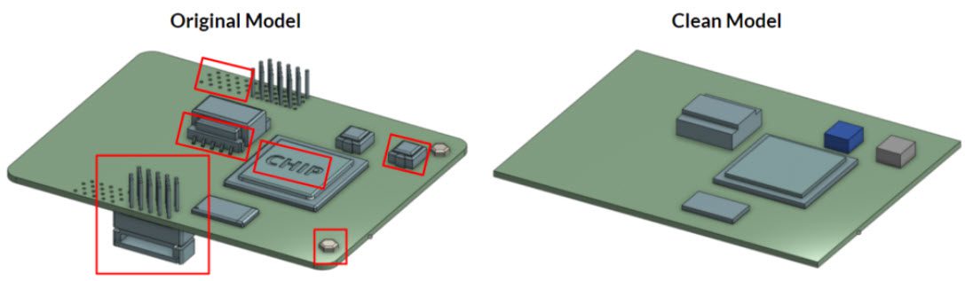
1. CAD Cleaning

Following points are essential:

• Firstly, avoid sheet/surface elements. The CAD model should only consist of solid parts.
• Secondly, avoid overlapping solids (unless they represent cell zones).
• Finally, avoid any CAD faults. This article explains how to find faults in your CAD.

Following points are not essential, but we strongly recommend to perform a cost-effective simulation experience:

• Model only the essential parts. In other words, remove extra or unnecessary features/components. (small nuts, bolts, pins, etc.).
• Fill leftover holes and gaps.

2. CAD Preparation

Imprint the CAD model. This will create individual faces for the contacts. Refer to this page to see what the imprint feature does. In addition, if you need to know more information regarding the CAD preparation, visit this page.

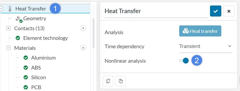
3. Material Assignment

If you would like to assign temperature-dependent material properties, activate Nonlinear Analysis.

Define the temperature-dependent material properties on a table:

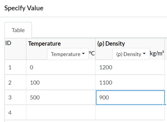
For more information about the table assignment, check this article.

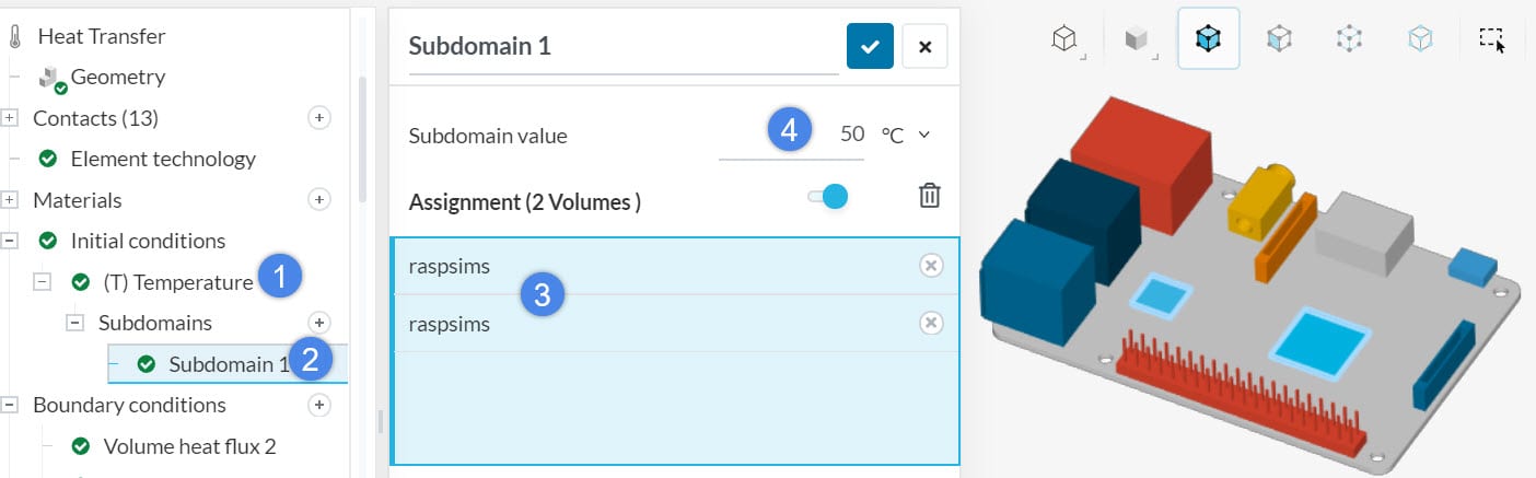
4. Initial Conditions

Define the initial temperature of the components. To clarify, the Temperature section is a quick way to assign temperature values on every component, without selecting them. Moreover, you can create a subdomain to define the initial temperature of individual components.

5. Boundary Conditions

You can find the available boundary conditions (BC) for heat transfer analysis on this page. In this article, you will learn about the commonly used BCs for transient heat transfer analysis.

5.1 Volume Heat Flux

Use this BC to define the heat-generating components. In a transient analysis, you can define the heat generation time-dependent.

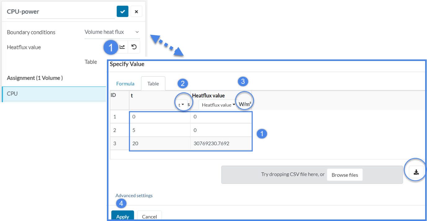
You can upload the data as a .csv file, or manually type it in the table. Do not forget to update the headers of the table.

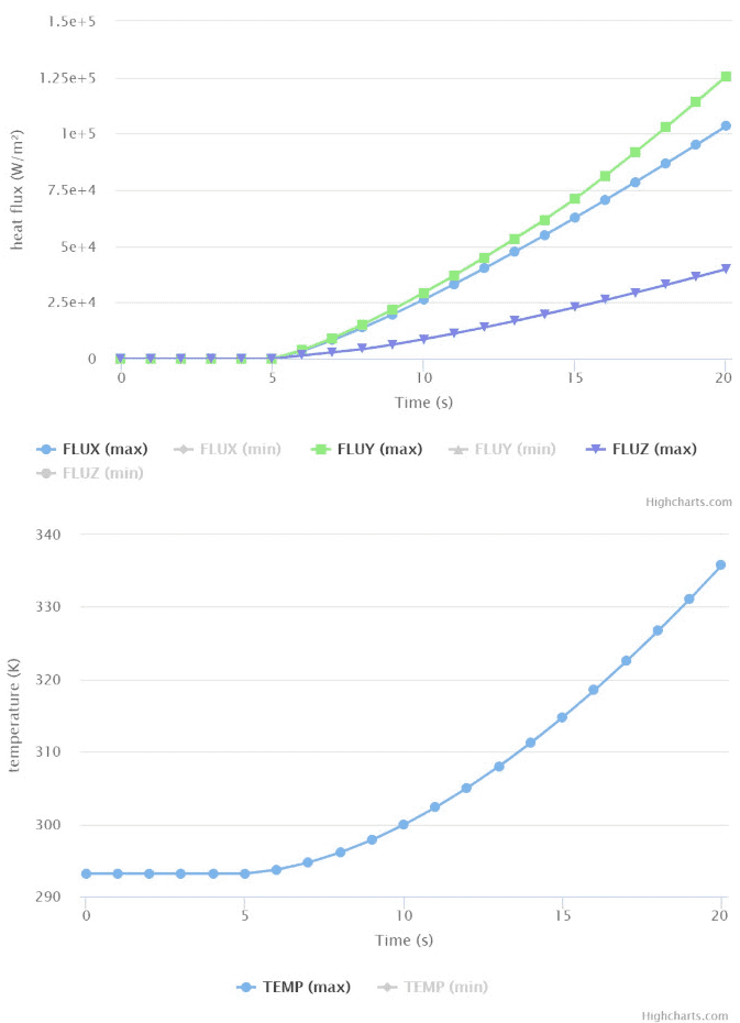
The table assignment above shows that there is no heat generation during the first 5 seconds. Starting by the second 5, heat generation begins and reaches to about 30.8 MW/m³ until 20 seconds. If you want heat generation to continues as 30.8 MW/m³ until the end of the simulation, add another row and define the end time and 30.8 MW/m³ . Otherwise, the corresponding heat generation values, which are not defined in the table, are found by extrapolation. Result of the given assignment is showed in the following charts:

5.2 Convective Heat Flux

Convective heat flux boundary condition can be used to define the heat exchange between the components and the surrounding environment. For instance, the heat exchange between a solid and ambient usually occurs with convective and radiation heat transfer.

You can use some benchmarks to find out convective and radiative heat transfer coefficients. Or perhaps, there is a solid layer, which is not modeled, on the selected heat transferring surface. In conclusion, no matter which heat transfer scenario takes place, you can assign the heat transfer coefficient and reference temperature to convective heat flux BC.

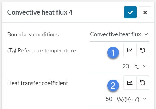
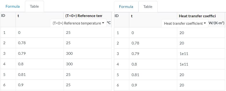
Similarly, you can define the heat transfer coefficient or reference temperature in a table. For example, you can define the reference temperature as a time-dependent value to simulate ambient temperature change.

Sudden heat input will result in a sudden temperature increase in the system. Sometimes the user only have temperature data from the measurements. In this case, it is not possible to assign a fixed temperature boundary condition and expect a sudden temperature increase and then let the system cool. However, you can use the Convective Heat Flux boundary condition. Just assign a very high heat transfer coefficient during the sudden heat input time, then reduce it afterward.

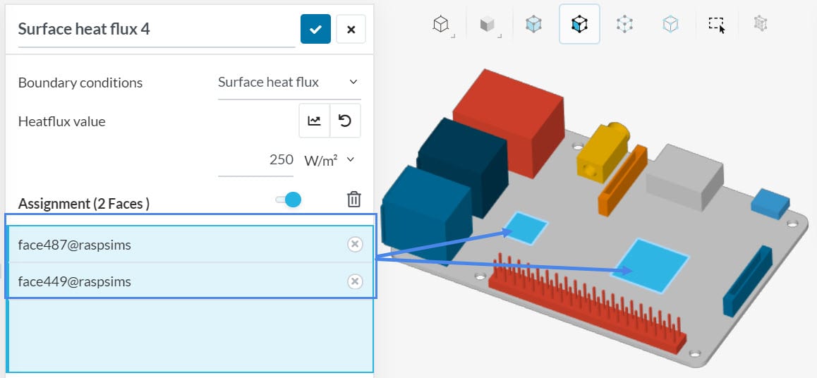
5.3 Surface Heat Flux

Surface heat flux can be used to define heat generation on a surface. For example, you may have some small circuit elements on PCB, which generates heat. You don’t need to model all these tiny elements. Just create the region they were placed as a separate area on CAD and assign surface heat flux in SimScale.

Another possible use of heat flux is to define the heat losses temperature-dependent. Just use empirical approximations or this website to approximate radiation and convective heat transfer coefficients.

$$U = h_{r} + h_{c} \tag{1}$$

where, \(U\) [W/m²-K] is overall heat transfer coefficient, \(h_{c}\) and \(h_{r}\) are convection and radiation heat transfer coefficients respectively.

$$q = U \cdot \Delta T \tag{2}$$

where, \(q\) [W/m²] is heat flux, and \(\Delta T\) [K] is temperature difference between the surface and its surrounding.

The table definition is important to achieve temperature-dependent heat flux. Especially in high-temperature differences between the surface and the external domain, radiative heat transfer effects are significant. The following table shows temperature-dependent heat loss from a horizontal flat surface. In this example, the surrounding domain is assumed as 20°C still air. Surface emissivity is assumed as 1 (black body).

6. Meshing

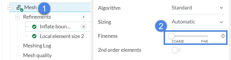
Usually, it is recommended to create 3 or 4 nodes per thickness. In transient simulations, mesh size significantly affect the simulation time and cost. Therefore, it might be challenging to achieve the mesh intensity you would like to achieve.

If you have a complex model with very thin parts, it is recommended to assign a very coarse fineness level, but add layer refinement. This is a cost-effective meshing method.

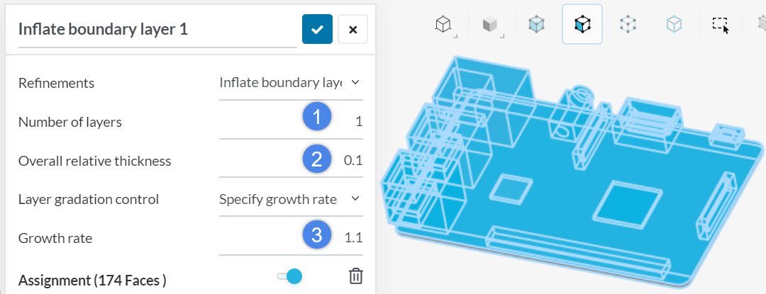
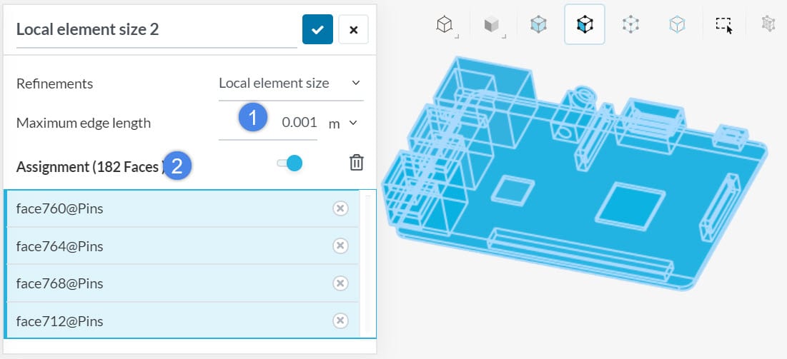
It is always a good idea to use a local element size refinement. This will help to control the mesh size and create a uniform mesh.

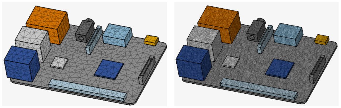
The following picture shows the results of two meshing strategies. Boundary layer and local element size refinements are the recommended meshing method.

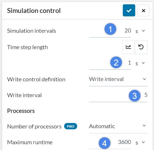
7. Time Step

You can use the default Numerics in your initial run. Simulation interval is the simulation time. Small time step length leads to more accurate results, but increase the computation time.

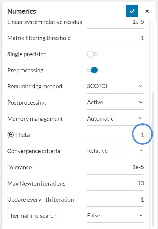
If you observe any instability in the results, the time step size might be too big. Under Numerics, change the theta value to 1 to use the Implicit method.

If the simulation fails with insufficient memory error or insufficient disks pace error, reduce the theta value (close to zero) and assign a small time step. The following equation defines the theoretical limitation of maximum time step length in the explicit method:

$$\Delta t = \frac{1}{2} \cdot \frac{\Delta x^2 \cdot \rho \cdot c_p}{\kappa} \tag{3}$$

Where, \(\Delta t\) \([s]\) is time step, and \(\Delta x\) \([m]\) is minimum cell size (distance between two nodes), \(\rho\) \([kg/m^3]\) is density, \(c_p\) \([J/kg-K]\) is specific heat capacity, and \(\kappa\) \([W/m-K]\) is the thermal conductivity of the material of interest.

Further Tips:

1. First, perform a simulation with a coarse mesh. Once you’ve got the results, increase the mesh intensity, and re-run the simulation. Finally, Compare the final simulation result with the previous one. Repeat this until the results are consistent.
2. Start the initial simulation with a large time step. Then reduce the time step length and re-run the simulation. Similarly, compare the results and follow the same procedure.