Validation Case: DrivAer Model

This validation case belongs to fluid dynamics. The aim of this validation case is to validate the lattice Boltzmann (LBM) solver by Pacefish®\(^3\) implemented in SimScale by conducting an aerodynamic study on 4 DrivAer car models. The following parameters are used for comparison:

• Drag coefficient (\(C_d\))
• Pressure coefficient (\(C_p\))

This validation case compares the simulation results done in SimScale with results presented in the studies [1] and [2].

Geometry

As mentioned before, this validation case uses 4 DrivAer car models. These models are publicly available models and serve as an effort to close the gap between simplified models, such as the Ahmed body, and highly complex models that are ready for production. The models used in this validation case can be seen in the figure below:

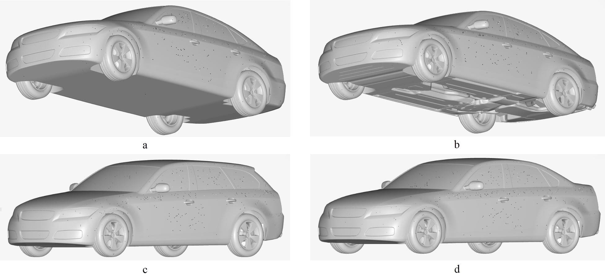
These 4 geometries have the same reference length of 4.6 \(m\) and a reference frontal area of 2.16 \(m^2\). These models were also placed in a virtual wind tunnel in the Workbench such as below:

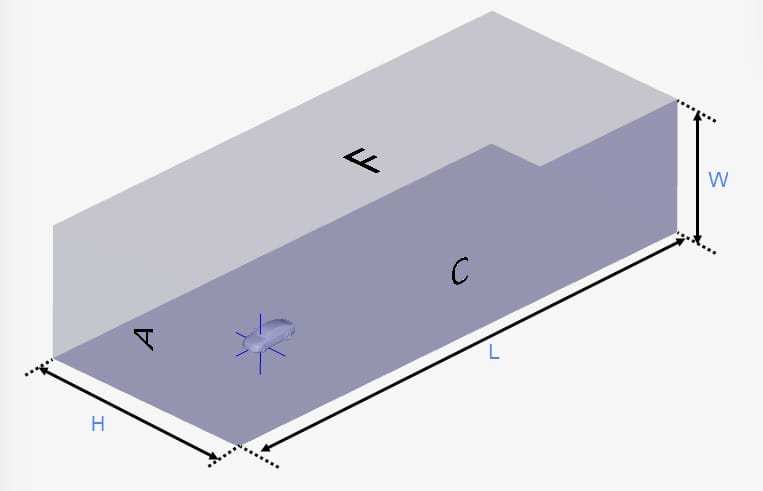
The dimension of the wind tunnel can be seen in the table below:

Length L \([m]\)	Width W \([m]\)	Height H \([m]\)	Blockage Ratio \([\phi]\)
48	20	12	1%

Analysis Type and Mesh

Tool Type: Lattice Boltzmann Method (LBM) (Pacefish\(^®\) by Numeric Systems GmbH)

Analysis Type: Transient incompressible and SST-DDES turbulence model

Mesh and Element Types:

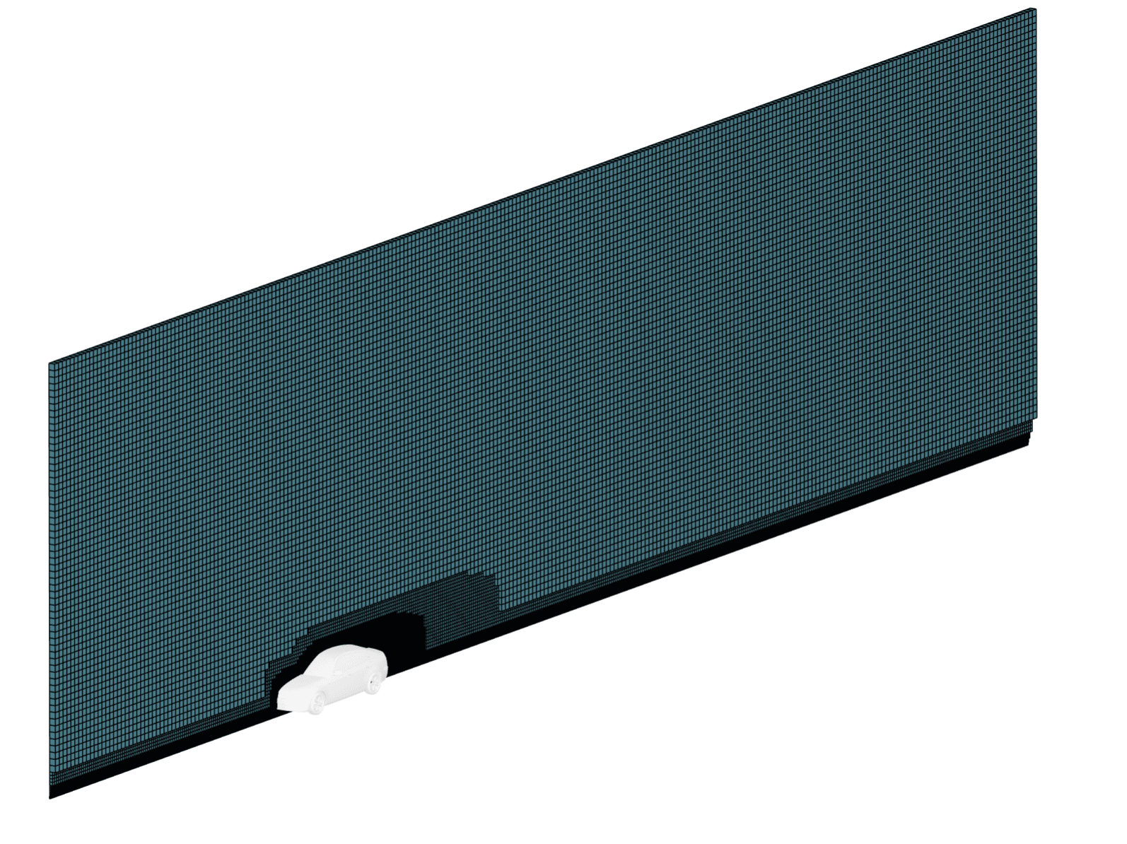
In order to get accurate results, the mesh for the fastback – smooth underbody model was generated using Manual mesh settings so that the reference length can be used to determine the sizing of the mesh, but the mesh settings for the other models used Automatic mesh settings. The details of the mesh for each model can be seen in the table below:

Model	Number of Cells	Minimum Cell Size \([mm]\)
Fastback – Smooth Underbody (a)	135 Million	2.2
Fastback – Detailed body (b)	162.2 Million	3
Estateback (c)	71.2 Million	4.5
Notchback (d)	162.2 Million	3

Also, refinements are automatically added in the direction of the flow to capture the wake accurately, an example of the mesh used in the simulation can be seen below:

Simulation Setup

Fluid:

• Air
  • Kinematic viscosity \((\nu)\): 1.567e-5 \(m^2/s\)
  • Density \((\rho)\): 1.184 \(kg/m^3\)
  • Reynolds number \((Re)\): 4.87e6

Boundary Conditions:

When using the LBM solver, the boundary conditions are assigned at the surfaces of the flow domain. The boundary conditions for this case can be seen in the table below:

Surface	Boundary Condition	Quantity
A	Velocity inlet – Fixed Magnitude	16 \(m/s\)
B	Pressure Outlet	–
C	Slip Wall	–
D	Slip Wall	–
E	Moving Wall	16 \(m/s\)
F	Slip Wall	–
Wheels	Rotating Wall	51 \(rad/s\)

Reference Solution

This case is validation against the reference result obtained through an experiment where the DrivAer car models are placed in a wind tunnel. The car model has a scale of 1:2.5 and the dimensions of the wind tunnel are:

L \([m]\)	W \([m]\)	H \([m]\)	Blockage ratio \([\phi]\)
4.8	2.4	1.8	8%

The wind tunnel also has a moving belt system that can move up to 50 \(m/s\). The body is held from above by a central strut and the wheels are held by four separate horizontal struts that are outside of the test section\(^1\).

The time-averaged pressure measurements were done by using a multiport measurement system. The sampling rate for this study was 20 Hz with an averaging period of 10 \(s\). There were 188 measurement points that were used in the study and they were distributed along the model surface\(^1\).

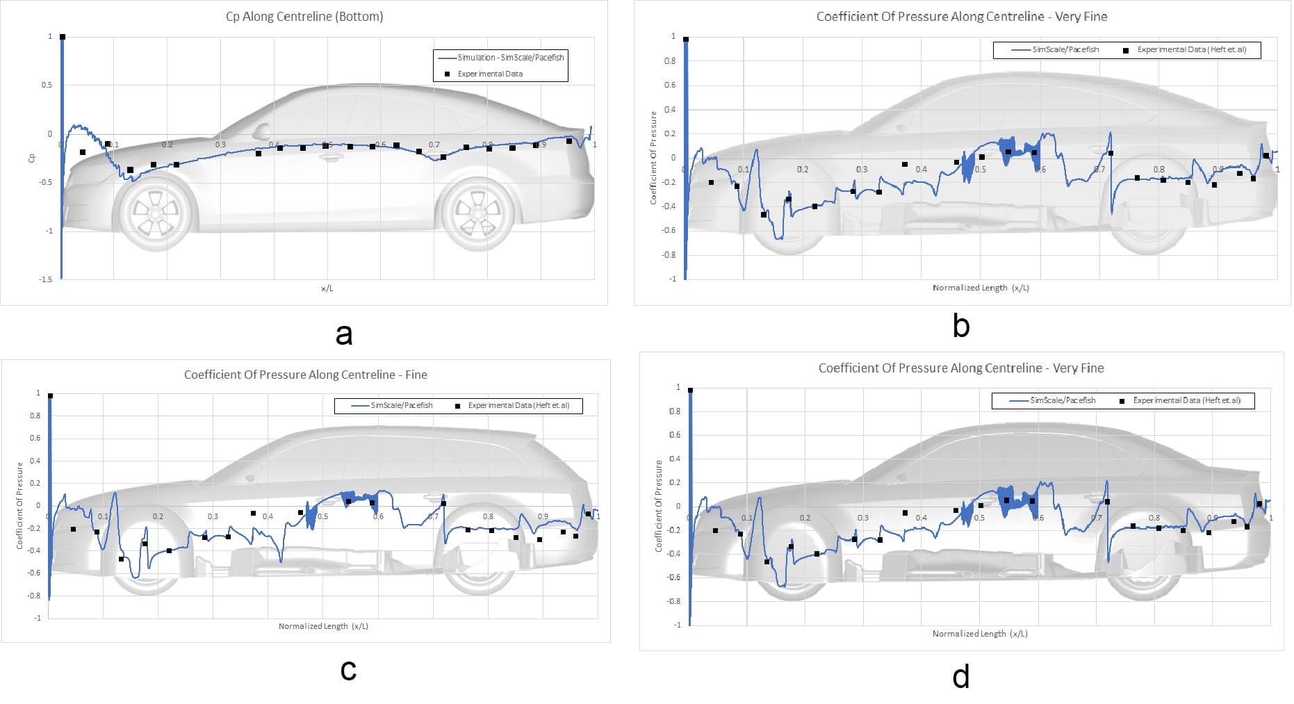
Result Comparison

As mentioned before, this validation case compares the pressure and drag coefficient obtained from SimScale against the experimental results obtained from the two studies referenced\(^{1,2}\).

1. Drag Coefficient (\(C_d\))

The drag coefficient for each car model were calculated with the following formula:

$$C_d = \frac{F}{\frac{1}{2}\rho\ U^2\ A}\tag{2}$$

where:

• \(F\): total force which consists of the pressure and friction force in the x-direction \((N)\).
• \(\rho\): fluid density (\(kg/m^3)\)
• \(U\): fluid velocity \((m/s)\)
• \(A\): reference area \((m^2)\)

The calculated drag coefficients from the simulation were then compared with the experimental results, which can be seen in the table below:

Car Model	Experimental	Simulation	Error [%]
Fastback – Detailed Underbody	0.275	0.268	2.55
Estateback	0.319	0.304	4.70
Notchback	0.277	0.271	2.24

2. Pressure Coefficient (\(C_p\))

To calculate the pressure coefficient, the pressure values at the top and bottom of the car surface along a centerline in the y-axis need to be extracted. This can be done by using the Forces and moments feature implemented in SimScale. Next, with the obtained pressure value, the pressure coefficient was calculated with the formula below:

$$C_p = \frac{p-p_{\infty}}{\frac{1}{2}\rho\ U^2}\tag{1}$$

where:

• \(p\): static pressure at the point of calculation \((Pa)\)
• \(p_{\infty}\): static pressure in the freestream \((Pa)\)
• \(\rho\): freestream fluid density \((kg/m^3)\)
• \(U\): freestream fluid velocity \((m/s)\)

The comparison of pressure coefficients for each car model along the centerline at the top and bottom can be seen in the figures below:

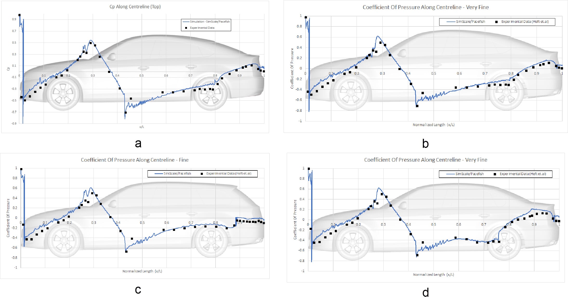
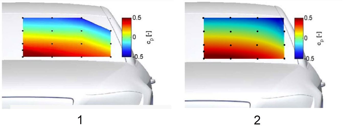
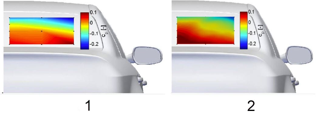
Furthermore, a detailed comparison of the pressure coefficient at the front windshield of the fastback model and at the back windshield of the notchback can be seen in the figures below:

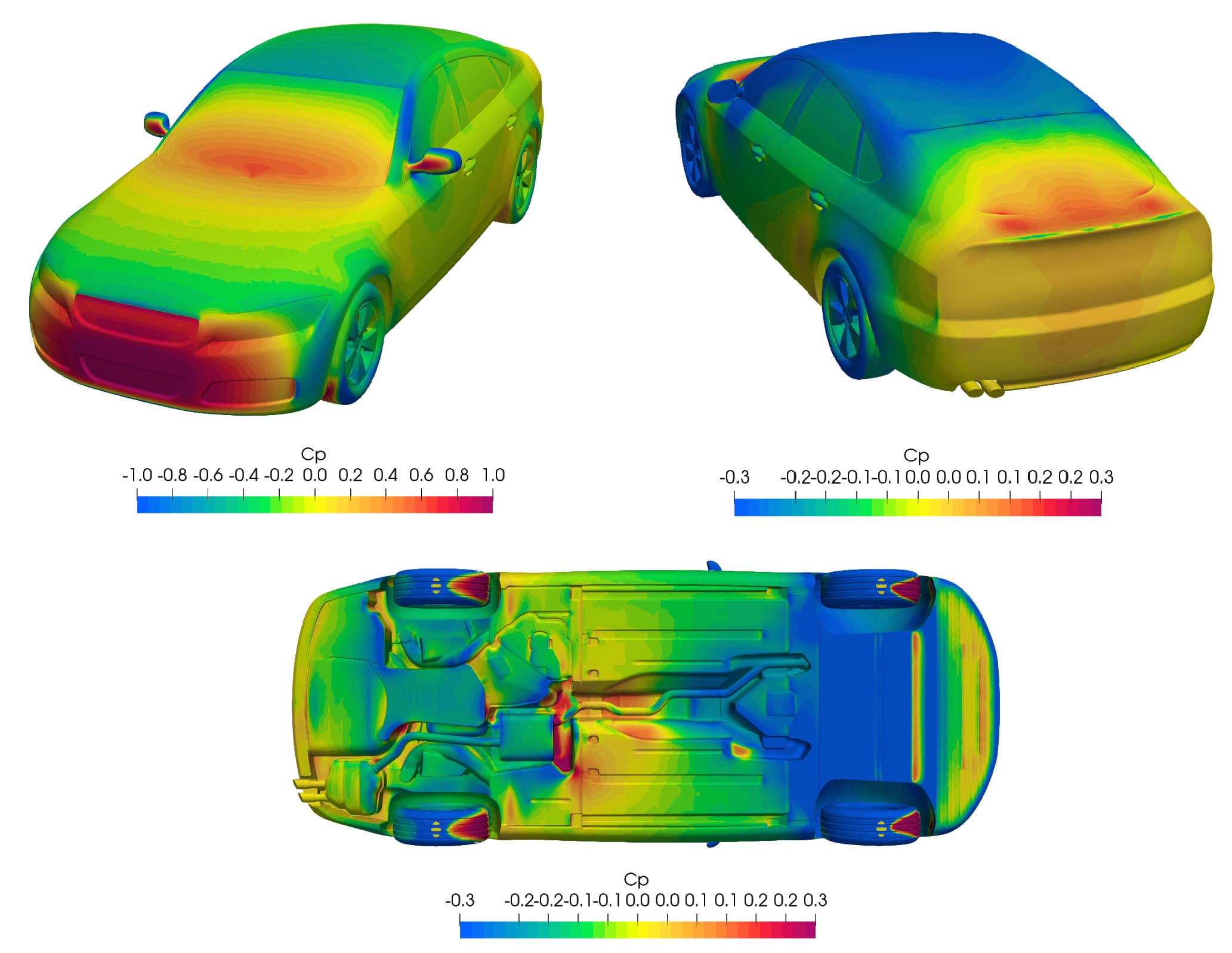
The pressure coefficient distribution around the fastback model as observed from simulations:

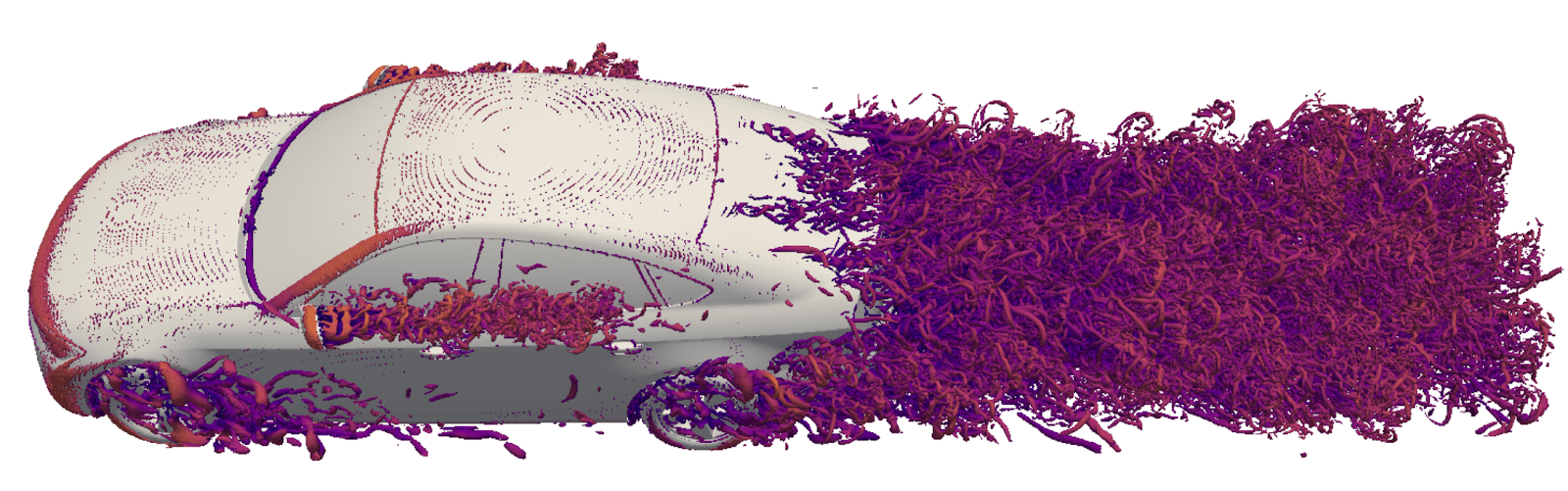
Transient Results

Transient data allows for a more in-depth understanding of the flow around the car models and enables the investigation of time-dependent effects. An image of the Q-criterion is given in Figure 9:

The transient variation in pressure, vorticity, and flow velocity around the estateback model are given in the animations below:

Related tutorials:

• Aerodynamic simulation of a truck

Last updated: February 2nd, 2023

References

- Heft et al. “Experimental and Numerical Investigation of the DrivAer Model”, 2012
- Heft et al. “Introduction of a new realistic generic car model for aerodynamic investigations”, 2012
- https://www.numeric.systems/