Validation Case: Non-Newtonian Flow Through Expansion Channel
The non-Newtonian flow through an expansion channel validation case belongs to fluid dynamics. This test case aims to validate the following parameter:
- Non-Newtonian fluid with the power law model
The simulation results of SimScale were compared to the analytical results presented in [Tanner, 1992 apud Manica]\(^1\).
Geometry
The geometry consists of a pseudo-2D channel, with a 3:1 expansion ratio, as seen in Figure 1:
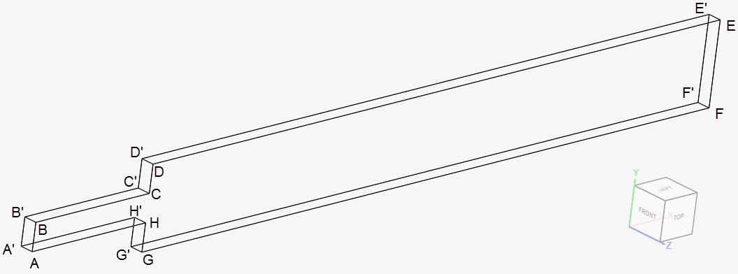
The dimensions of the channel are given in Table 1:
| A | B | C | D | E | F | G | H | |
| x \([m]\) | 0 | 0 | 5 | 5 | 30 | 30 | 5 | 5 |
| y \([m]\) | -0.5 | 0.5 | 0.5 | 1.5 | 1.5 | -1.5 | -1.5 | -0.5 |
| z \([m]\) | 0.25 | 0.25 | 0.25 | 0.25 | 0.25 | 0.25 | 0.25 | 0.25 |
The corresponding nodes marked with an apostrophe (‘) are translated 0.5 m along the negative z-direction.
Note
SimScale requires a domain with volume to perform simulations. Therefore, we are going to use a pseudo-2D approach for this validation case.
The meshes used in this project contain a single cell along the z-direction. An empty 2D boundary condition will be applied to both sides of the domain, so the z-direction won’t be resolved.
Analysis Type and Mesh
Tool Type: OPENFOAM®
Analysis Type: Steady-state incompressible flow
Turbulence Model: Laminar
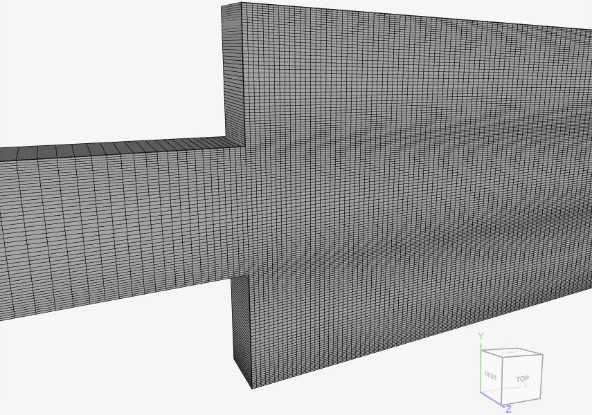
Mesh and Element Types: Both meshes used in this validation case are hexahedral meshes created locally and imported to SimScale. Cases A through D were run with an intermediate fineness mesh (30700 cells) and with a fine mesh (77600 cells).
In Table 2, an outline of the cases is presented, including information regarding the mesh and the power-law model parameters.
| Case | Mesh Type | Cells | Element Type | \(K\ [m^2/s]\) | \(N\) | \(\nu_{min}\ [m^2/s]\) | \(\nu_{max}\ [m^2/s]\) |
| (A) | blockMesh | 30700 – 77600 | 3D hexahedral | 0.008838835 | 0.5 | 0.000001 | 0.5 |
| (B) | blockMesh | 30700 – 77600 | 3D hexahedral | 0.0125 | 1 | 0.000001 | 0.5 |
| (C) | blockMesh | 30700 – 77600 | 3D hexahedral | 0.01767767 | 1.5 | 0.000001 | 0.5 |
| (D) | blockMesh | 30700 – 77600 | 3D hexahedral | 0.025 | 2 | 0.000001 | 0.5 |
Find below the 30700 cells intermediate fineness hexahedral mesh. It contains a single cell in the z-direction.
Simulation Setup
Material:
- Viscosity model: Power law non-Newtonian model, with coefficients as described in Table 2;
- \((\rho)\) Density: 1 \(kg/m^3\).
Note
In the non-Newtonian model, fluids with \(N\) < 1 are called shear thinning or pseudoplastic fluids. As examples, we have paint, blood, and ketchup.
Fluids with \(N\) > 1 are referred to as shear thickening or dilatant fluids. Oobleck (mixture of cornstarch and water) is an example of shear thickening fluid.
Lastly, for \(N\) = 1, we have a Newtonian fluid. Therefore, three types of fluids are evaluated in this validation case.
Boundary Conditions:
Before defining the boundary conditions, the current nomenclature will be used for the rest of this documentation:
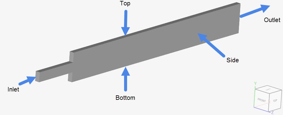
In the table below, the configuration for both velocity and pressure are given at each of the boundaries:
| Boundary type | Velocity \([m/s]\) | Pressure \([Pa]\) | |
| Inlet | Velocity inlet | Fixed value: 0.5 in the x-direction | Zero gradient |
| Outlet | Pressure outlet | Zero gradient | Fixed value: 0 |
| Sides | Empty 2D | Empty 2D | Empty 2D |
| Top and bottom | Wall | Fixed value: 0 | Zero gradient |
Reference Solution
A dimensionless analytical solution for the developed velocity profiles within a channel is presented by Tanner [Tanner, 1992 apud Manica]\(^1\).
Result Comparison
The numerical simulation results for the various power indexes \(N\), ranging from 0.5 to 2, are compared with the analytical solution. For all cases, the Reynolds number was kept at 40.
The generalized Reynolds number formulation for non-Newtonian flows is as follows (SI units apply for all parameters):
$$Re=\frac{\rho\ V^{2-N} H^{N} }{K} \tag{1}$$
Where:
- \(\rho\) is the density;
- \(V\) is the flow inlet velocity;
- \(H\) is the inlet height;
- \(N\) is the power index from the power law formulation;
- \(K\) is the consistency factor from the power law formulation. The consistency factor was adjusted for each case, to maintain \(Re\) = 40.
Cases A through D were run with both intermediate and fine meshes. The presented results are those from the intermediate mesh, as no further improvement was observed with the finer discretization.
The figure below shows the normalized velocity profiles in the fully developed region downstream of the expansion, at \(x\) = 28 \(m\). The \(y\) coordinates, represented in the horizontal axis of Figure 4, are normalized from 0 (center of the channel) to 1 (top of the channel).
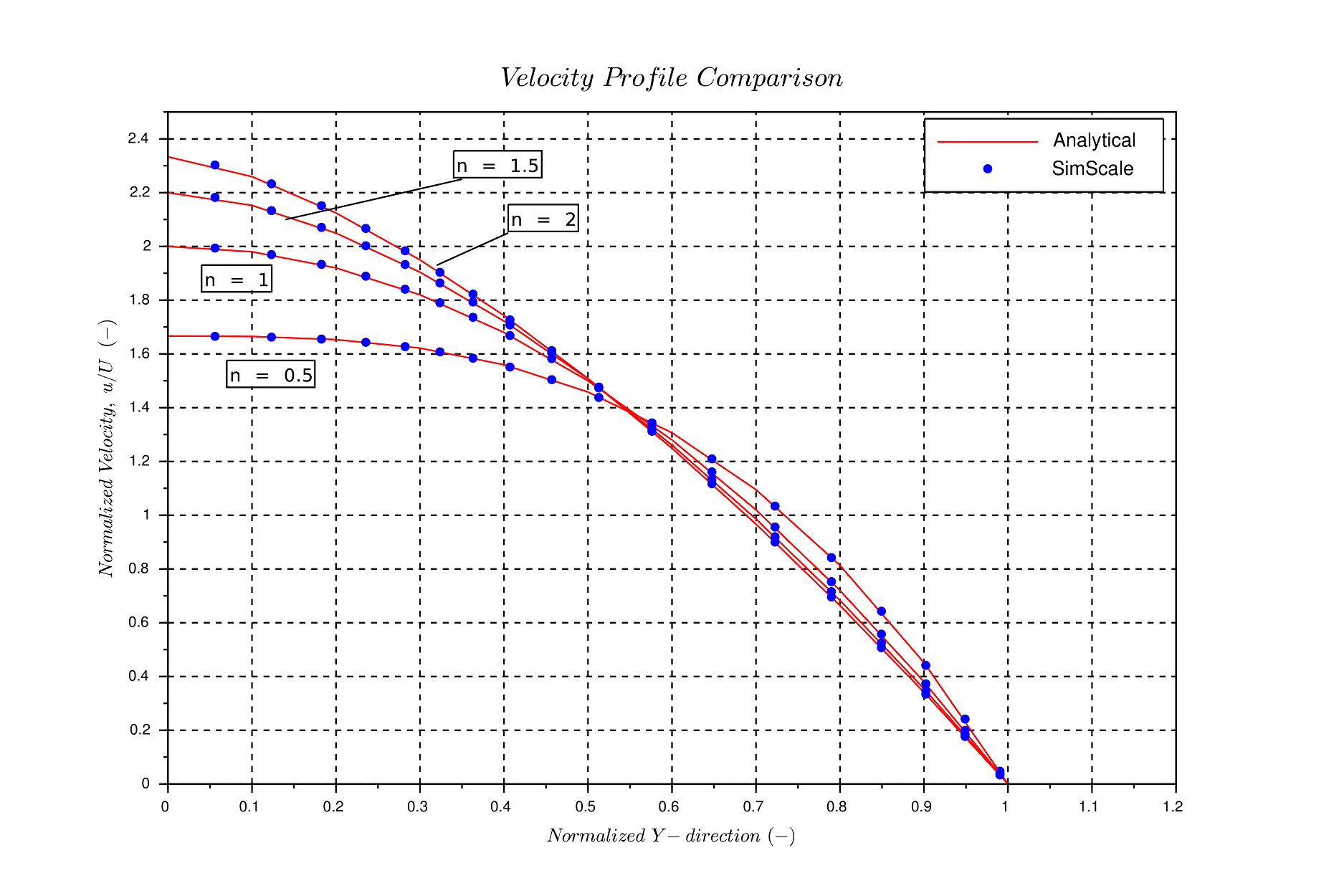
Note that, in the figure above, ‘n’ represents the same power index \(N\) used within the workbench.
SimScale’s results show very good agreement with the analytical solution for all configurations.
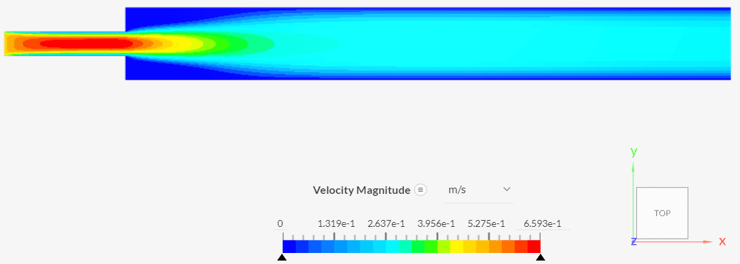
In Figure 5, we can see how the velocity profile is developing along the expansion channel for case A (\(N\) = 0.5) with the intermediate fineness mesh.
Last updated: November 7th, 2023
Did this article solve your issue?
How can we do better?
We appreciate and value your feedback.


