Non-Newtonian Models
Non-Newtonian models are used to model the behavior of non-Newtonian fluids in CFD simulations. On this page, the most commonly used non-Newtonian models available on the SimScale platform are described in detail.
Non-Newtonian Fluid
In a non-Newtonian fluid, the local shear stresses and the local shear rates in the fluid have a non-linear relation, where a proportionality constant can not be defined. Therefore, the viscosity is not a fixed scalar but a variable. Further, it is also important to note that the viscosity can be dependent on the shear rate or the time history of the shear rate.
Some examples are fluids like ketchup, custard, toothpaste, starch suspensions, paint, blood, and shampoo. Some of these fluids become runnier when shaken while some become more viscous.
Workbench
Currently, non-Newtonian fluids are only available for incompressible, multiphase, and convective heat transfer (incompressible) analysis types. Just go to Materials, select a material from the library, and choose a Viscosity model that you would want to use from the drop-down.
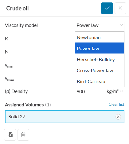
Figure 1 shows the general types of non-Newtonian fluids and their stress-strain behavior.
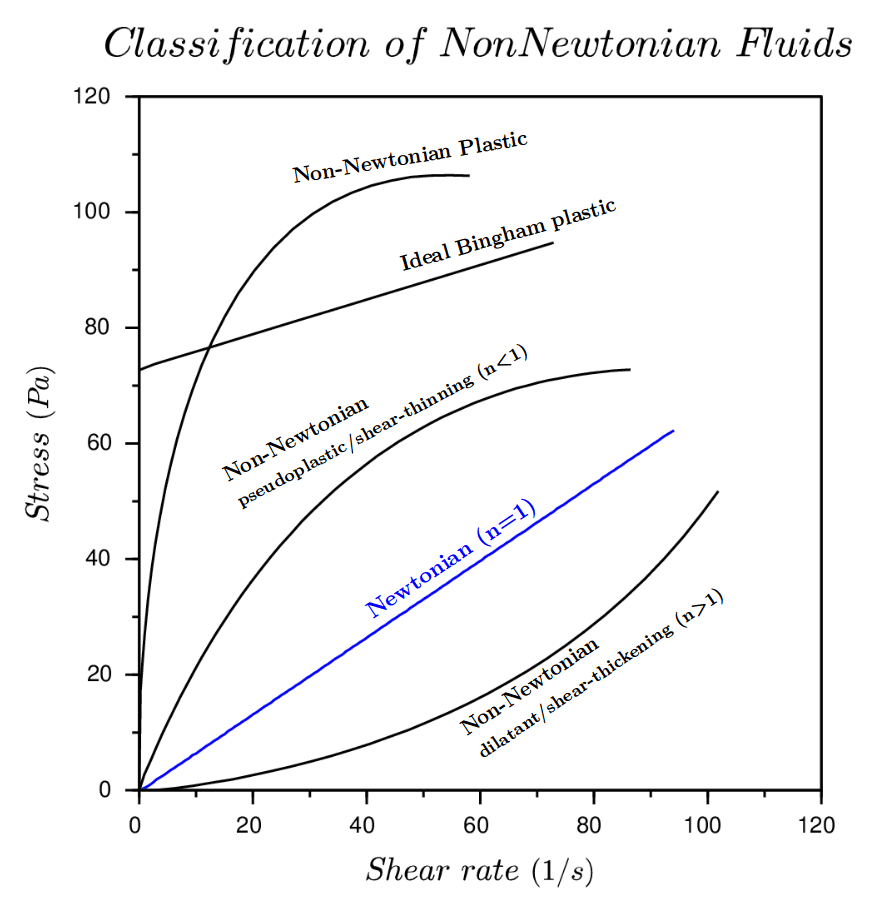
The 3 main types of non-newtonian fluids are briefly described as follows:
Pseudo-Plastic or Shear-Thinning Fluids
The pseudo-plasticity or shear-thinning behavior is described as a decrease in the viscosity of the fluid with an increase in the shear rate. Some common substances that undergo shear-thinning are ketchup, nail polish, silicone oil, and whipped cream.
Dilatant or Shear-Thickening Fluids
The dilatant or shear-thickening behavior is then described as being opposite to shear-thinning. That means an increase in fluid viscosity with an increase in the shear rate, hence also called ‘thickening’ fluids. A common example of a thickening or dilatant fluid substance is a corn-starch solution in water.
Visco-Plastic Fluids
For this type of behavior, there is a minimum stress threshold, called ‘yield stress’, that must be exceeded for the fluid to flow or deform. A visco-plastic fluid material will deform elastically (like a rigid body) if the external stress is less than the yield stress value. When the external stress is greater than the yield stress, the relation between stress and strain rate may be linear or nonlinear.\(^2\)
Note
A visco-plastic fluid with a linear behavior is called a “Bingham plastic fluid” that has a constant viscosity (coefficient of proportionality) and constant yield stress.
Non-Newtonian Models
The available mathematical models that describe the relationship between shear stress and shear rate of non-Newtonian fluids are as follows:
Important
Please note that all models use the kinematic viscosity, \(\nu\).
1. Power Law Model
The Power law fluid model is a type of generalized model. It gives a basic relation for viscosity, \(\nu\), and the strain rate, \(\dot{\gamma}\). In this model, the value of viscosity can be bounded by a lower bound value, \(\nu_{min}\), and an upper bound value, \(\nu_{max}\).
The relation is given as:
$$\nu=k\cdot\dot{\gamma}^{n-1} \tag{1}$$
Where, in SI units,
- \(k\) is the flow consistency index \([m^2/s]\),
- \(\dot{\gamma}\) is the shear strain rate \([s^{-1}]\),
- \(n\) is the flow behavior index.
Based on the flow behavior index, \(n\):
- if \(0 < n < 1\): The fluid shows pseudo-plastic or shear-thinning behavior. Here a smaller value of \(n\) means a greater degree of shear-thinning.
- if \(n=1\): The fluid shows Newtonian behavior.
- if \(n>1\): The fluid shows dilatant or shear-thickening behavior with a higher value of \(n\) resulting in greater thickening.
Did You Know?
Power law is the simplest model that approximates the behavior of a non-Newtonian fluid. Its limitations are that it is valid over only a limited range of shear rates. Therefore, the values of \(K\) and \(n\) are dependant on the range of shear rates taken into account\(^2\).
Yet, Power law is the most commonly and widely used model dealing with process engineering. applications.
2. Bird-Carreau Model
This is a four-parameter model that is valid over the complete range of shear rates. For cases where there are significant variations from the Power law model i.e., at very high and very low shear rates, it becomes essential to incorporate the values of viscosity at zero shear, \(\nu_{0}\), and at infinite shear, \(\nu_{∞}\) into the formulation.\(^2\)
For this model, the viscosity, \(\nu\), is related to the shear rate, \(\dot{\gamma}\), by the following equation:
$$\nu =\nu_{\infty}+(\nu_{0}-\nu_{\infty})\times [1+(k\cdot \dot{\gamma})^{a}]^{(n-1)/a} \tag{2}$$
Where,
- \(a\) has a default value of 2. It corresponds to the change from linear behavior to power law.
- \(\nu_{0}\) is the viscosity at zero shear rate.
- \(\nu_{\infty}\) is the viscosity at infinite shear rate.
- \(k\) is the relaxation time in seconds.
- \(n\) is the power index.
It can be seen from equation 2 that at a low shear rate, Carreau fluid behaves as a Newtonian fluid and at a high shear rate as a Power law fluid.
Note
The Bird-Carreau model is mostly used for food, beverages and also blood flow applications.
3. Cross-Power Law Model
The Cross-Power law model is also a four parameter model that covers the entire shear rate range.
The model formulation is given as:
$$\nu =\nu_{\infty}+\frac{(\nu_{0}-\nu_{\infty})}{1+(m\cdot \dot{\gamma})^{n}} \tag{3}$$
Where,
- \(\nu_{0}\) is the viscosity at zero shear rate.
- \(\nu_{\infty}\) is the viscosity at infinite shear rate.
- \(\dot{\gamma}\) is the shear strain rate \([s^{-1}]\).
- \(n\) is flow index.
- \(m\) is the natural time in seconds at which the linear behavior changes to a power law.
This model reduces to a Newtonian fluid behavior as \(m\) approaches zero value.
4. Herschel-Bulkley Model
The Herschel–Bulkley model is also a generalized, non-linear model of non-Newtonian fluids. This model combines the behavior of Bingham and power-law fluids in a single relation. For very low strain rates, the material behaves as a very viscous fluid with viscosity, \(\nu_{0}\). After a minimum value of strain-rate corresponding to a threshold stress \(\tau_{0}\), the viscosity is represented by the power-law relation.
The model formulation is given as:
$$\nu = min(\nu_{0}, \tau_{0}/\dot{\gamma} + k\cdot \dot{\gamma}^{n-1}) \tag{4}$$
with $$\tau=\tau_0+k\cdot \dot{\gamma}^{n}$$
Where, in SI units,
- \(\tau\) is the shear stress \([m^2/s^2]\).
- \(\tau_{0}\) is the yield stress \([m^2/s^2]\).
- \(k\) is the consistency index \([m^2/s]\).
- \(n\) is the flow index.
- \(\nu_{0}\) is the viscosity at zero shear rate.
Further, if \(\tau < \tau_{0}\) the Herschel-Bulkley fluid behaves as a non-deformable solid and not fluid. Again, based on the flow behavior index, \(n\):
- if \(0<n<1\): The fluid shows pseud-plastic or shear-thinning behavior.
- if \(n=1\) and \(\tau_{0}=0\): The fluid shows Newtonian behavior.
- if \(n>1\): The fluid shows dilatant or shear-thickening behavior.
Related Projects
References
- https://cfd.direct/openfoam/user-guide/transport-rheology
- Continuum Mechanics-Progress in Fundamentals and Engineering Applications, Dr. Yong Gan.
Last updated: May 22nd, 2025
Did this article solve your issue?
How can we do better?
We appreciate and value your feedback.


