Documentation
This tutorial showcases how to use SimScale to run a transient incompressible fluid simulation of a water turbine using rotating zones. The turbine in use is the Francis turbine.
Simulations involving rotating regions require a few additional steps during CAD preparation and simulation setup. We will cover the entire workflow in this tutorial.

This tutorial teaches how to:
We are following the typical SimScale workflow:
To begin, click on the button below. It will copy the tutorial project containing the geometry into your Workbench.
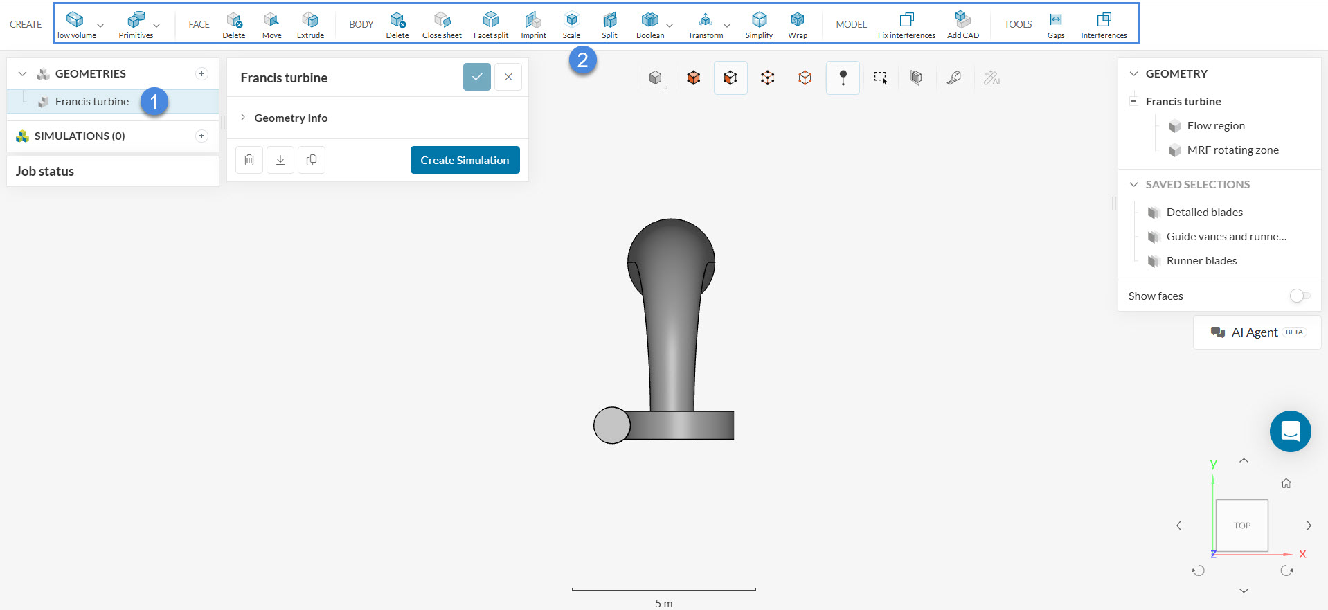
The following picture demonstrates what is visible after importing the tutorial project.
The geometry consists of the flow region of a Francis turbine. Furthermore, there’s also a solid cylinder part named Rotating zone.
Did you know?
Water turbines operate by removing kinetic and potential energy from the flow and converting it into mechanical torque on a shaft.
Water pumps work in the exact opposite way. By inputting mechanical energy, in the form of torque on a shaft, pumps can pressurize the water flow.
The imported geometry for this tutorial is ready for CFD simulations. Please note that it doesn’t contain any of the solid walls of the turbine. For this kind of analysis, only the flow region and rotating zone are necessary. In this tutorial, we’ll be using the prepared CAD model already. If we needed to make any modifications or to create a flow region from solid walls, we’d need to use the CAD environment. To modify a CAD model, simply select the geometry from the list—the available CAD operations will then appear in the top toolbar. You can either work directly on the original model or create a duplicate and apply your changes to the copy.
In case you are interested in the workflow to prepare your turbine design for a simulation with rotating zones, consider checking the following articles:
Select the Francis turbine geometry to open up the dialog box as in Figure 3:
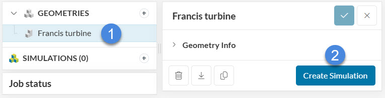
Hit the ‘Create Simulation’ button to open the simulation type selection widget:
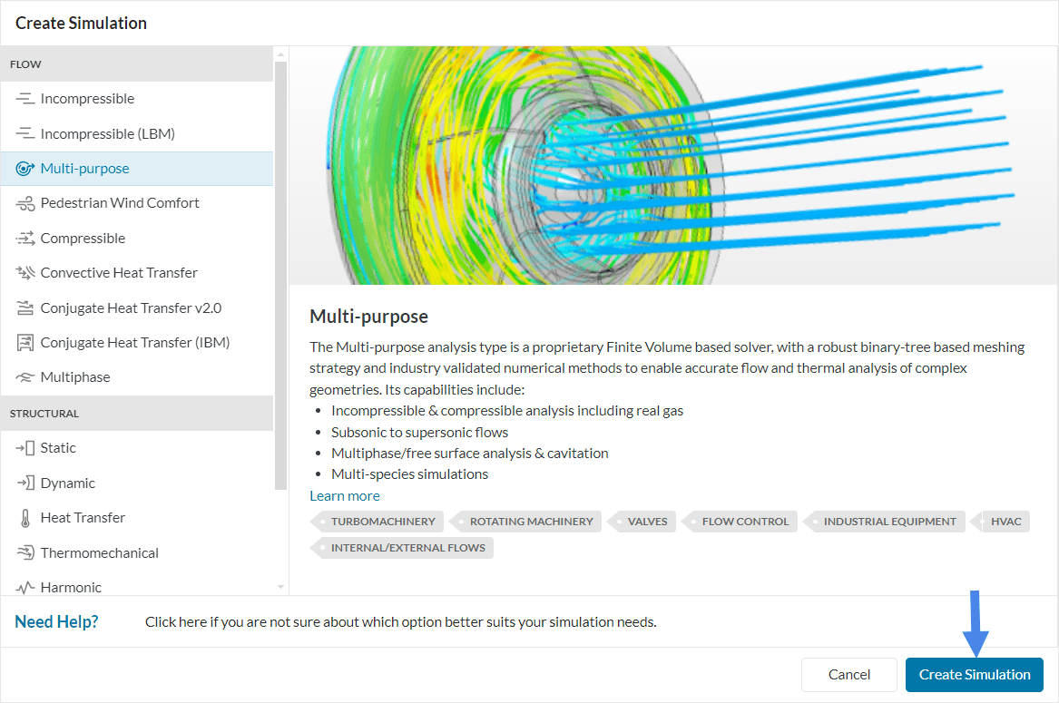
Choose ‘Multi-purpose’ as the analysis type and ‘Create Simulation‘.
At this point, the simulation tree will be visible in the left-hand side panel. To run the simulation, it’s necessary to configure the simulation tree entries.
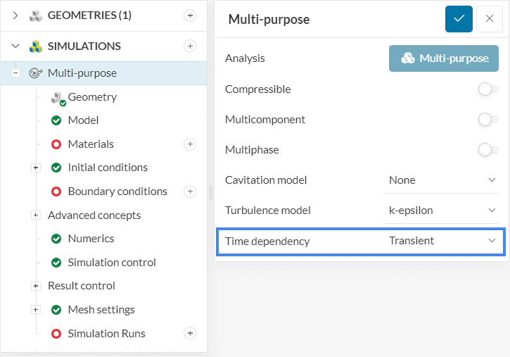
The global simulation settings remain as default, except for the Time dependency which should be changed to Transient as in Figure 5. This is because we are interested in the time-dependent variation of the quantities involved in flow physics. This also means that we will be dealing with sliding mesh for the rotating zone region.
Did you know?
Within the turbine blades, the flow experiences separation which is effectively captured by the k-epsilon turbulence model.
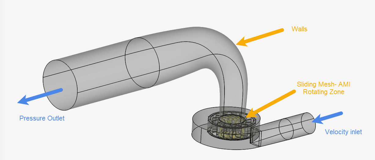
The following picture shows an overview of the boundary conditions.
For the current scenario, we will include the gravitational acceleration effects into the flow physics as well.
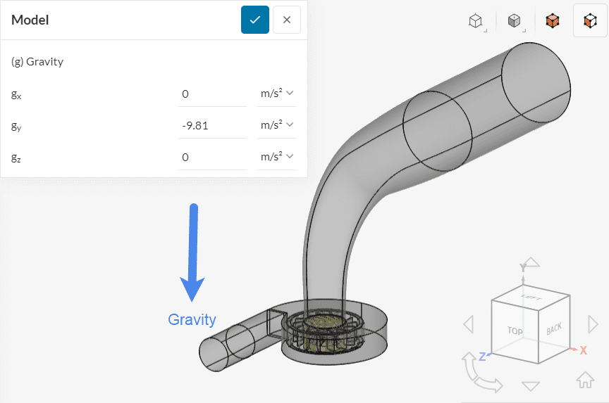
Click on ‘Model’ from the simulation tree and set gy to ‘-9.81’ \(m/s^2\).
This simulation will use water as a material. Therefore click on the ‘+ button’ next to Materials . In doing so, the SimScale fluid material library opens, as shown in the figure below:
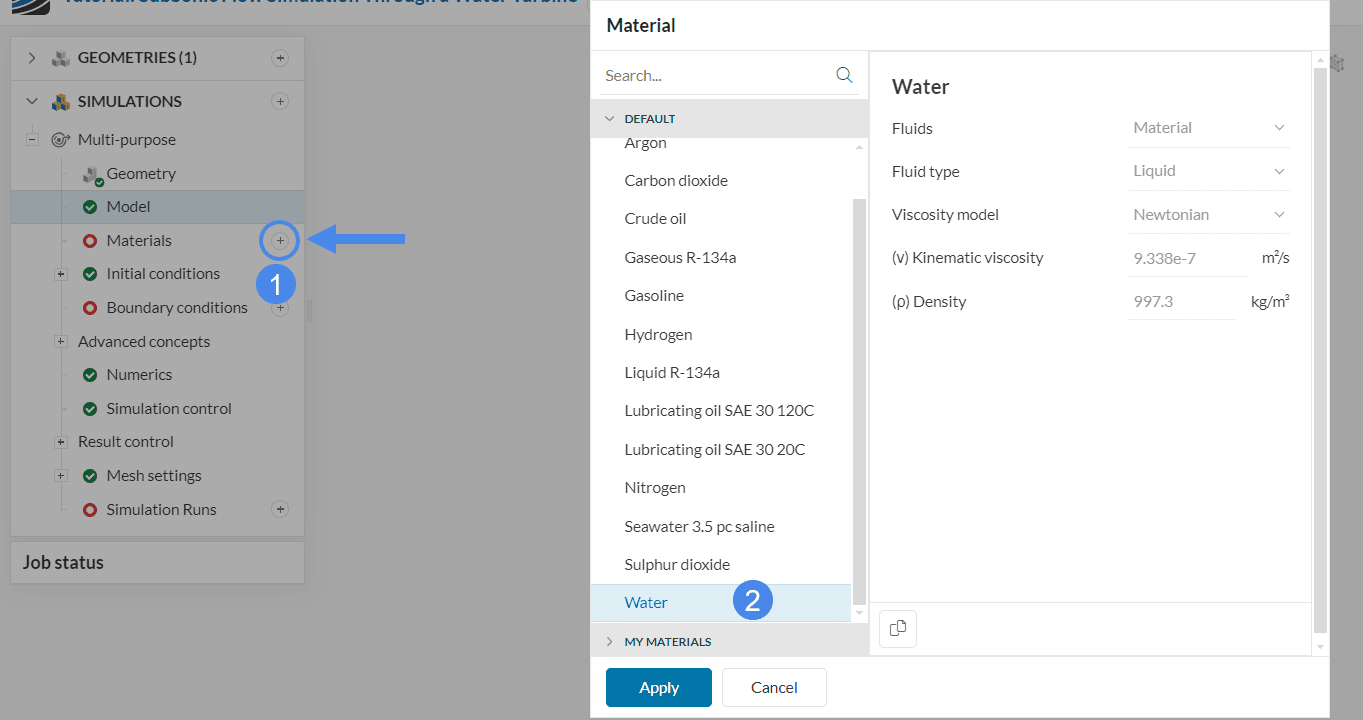
Select ‘Water’ and click ‘Apply’. Keep the default values, and assign the entire Flow region to it.
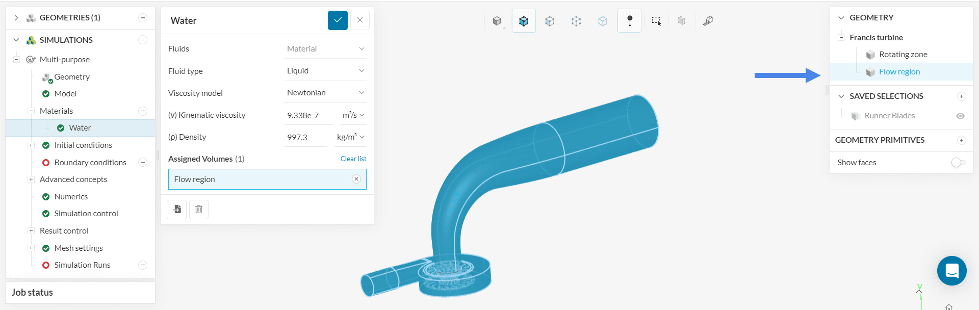
The Rotating zone volume is not assigned to any material.
In the next step, boundary conditions need to be assigned as shown in Figure 6. We have a velocity inlet and a pressure outlet. The rest are walls assigned by default.
a. Velocity Inlet
Click on the ‘+ button’ next to boundary conditions. A drop-down menu will appear, where one can choose between different boundary conditions.
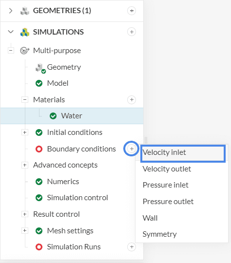
After selecting ‘Velocity inlet’, the user has to specify some parameters and assign faces. Please proceed as below:
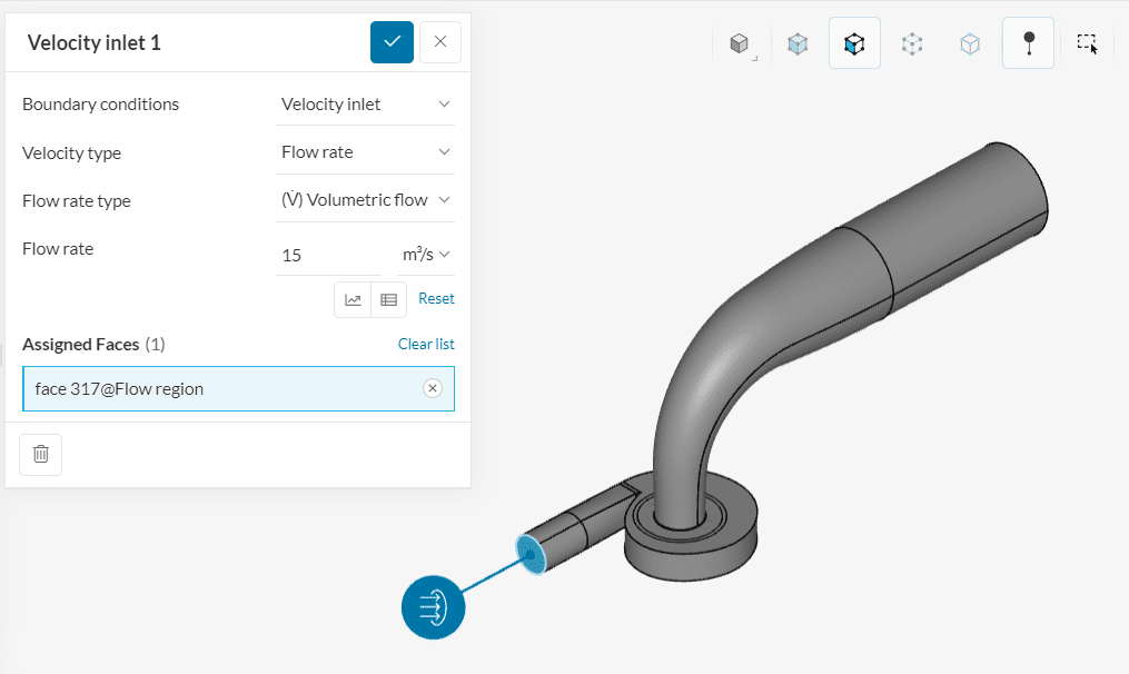
Water will enter through the inlet face at a volumetric flow rate of ’15’ \(m^3/s\).
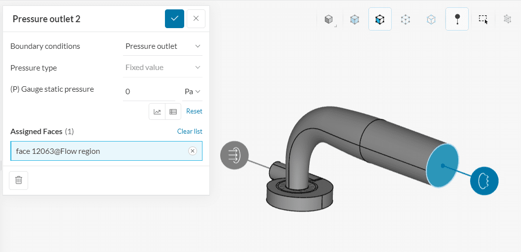
b. Pressure Outlet
Create a new boundary condition, this time a ‘Pressure outlet’, and select the outlet face. Make sure (P) Gauge static pressure is set to a fixed value of ‘0’ \(Pa\).
Did you know?
After going through the turbine runner, water exits through a section named draft tube. The purpose of this tube is to slow down the flux, converting kinetic energy into potential energy. The draft tube should be carefully designed, as it is directly related to kinetic energy loss at the outlet.
c. Walls
In Multi-purpose analysis, all the surfaces that act as walls are automatically treated likewise by the solver itself. Walls outside the rotating zone receive a no-slip condition and walls inside the rotating zone are treated as rotating walls unless you specifically pick the faces inside the rotating zone that you want to be static.
Did you know?
The entire volume inside the MRF rotating zone is spinning at a specified rotational velocity.
In case the rotating zone intersects a surface that shouldn’t be spinning, apply a no slip boundary condition.
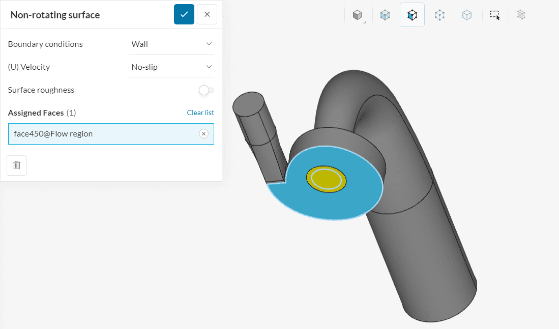
For example, in our geometry, one face that shouldn’t spin is intersected by the rotating zone:
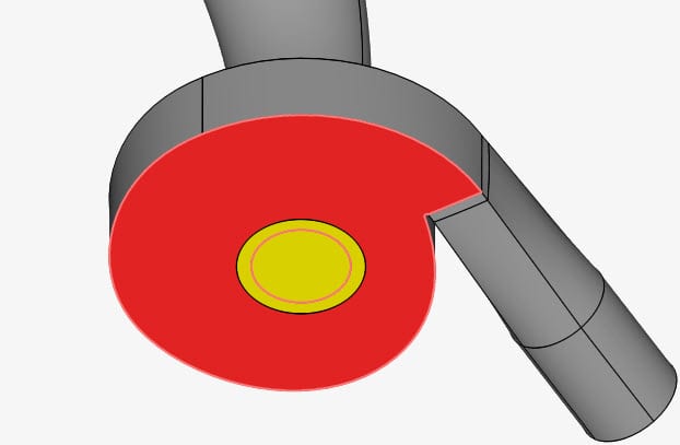
Apply a No-slip wall boundary condition to the bottom surface of the casing that is intersected by the rotating zone. This will ensure that the bottom face doesn’t spin despite being a part of the rotating zone.
In the simulation tree, navigate to Advanced concepts. Click on the ‘+ button’ next to Rotating zones. For transient simulations, this will actually model the sliding mesh zone. Define the sliding mesh zone (MRF) as shown:
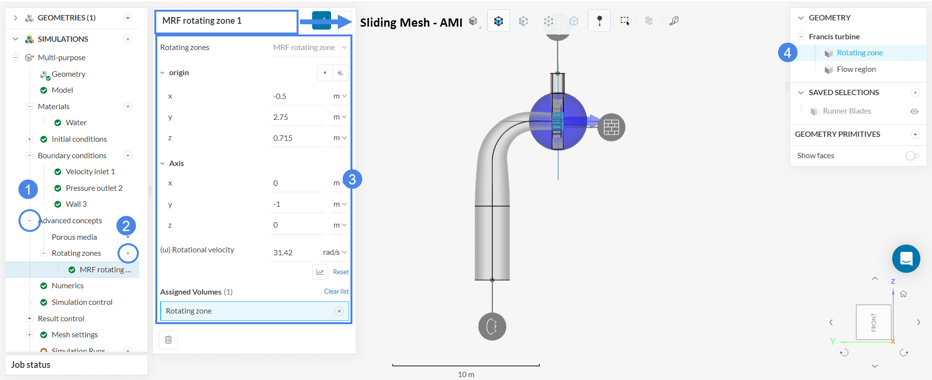
Note that the name of the rotating zone settings can be changed as required. When the time dependency is transient in Multi-purpose simulation, MRF already works as AMI. In the finished project attached at the bottom, MRF rotating zone has been set to Sliding Mesh – AMI to correspond with our setup, as shown above.
Did you know?
Note that the name of the rotating zone settings can be changed as required. When the time dependency is transient in Multi-purpose simulation, MRF already works as AMI. In the finished project attached at the bottom, it has been set to Sliding Mesh – AMI to correspond with our setup, as shown above.
No additional input is required when setting up the transient rotating zone for Multi-purpose simulations.
This article provides more information about the difference between MRF and AMI Rotating Zones.
Don’t worry about the numerical settings for the Multi-purpose simulations, as their default values are optimized. Open the simulation control settings and change the following:
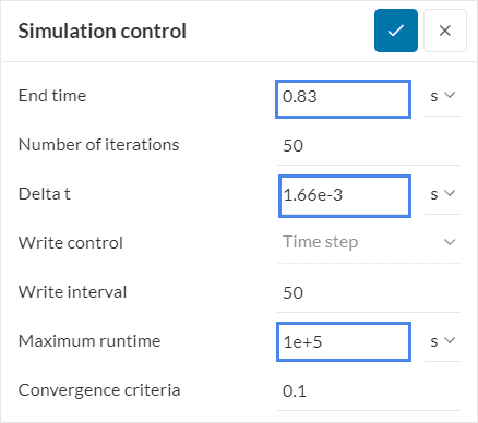
Keep the remaining settings as default. To know more about how to control the simulation read in detail here.
Result control allows you to observe the convergence behavior globally as well as at specific locations in the model during the calculation process. Hence, it is an important indicator of the simulation quality and the reliability of the results.
a. Forces and Moments
For this simulation, please set a ‘Forces and moments’ control on the Runner Blades as demonstrated in the picture below:
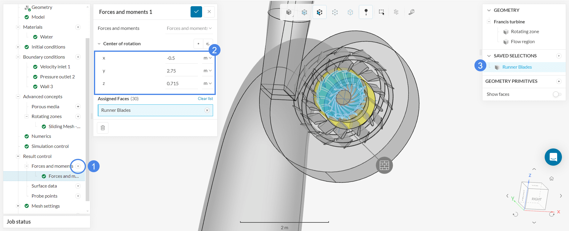
To save time, there’s a pre-saved saved selection for the runner blade surfaces.
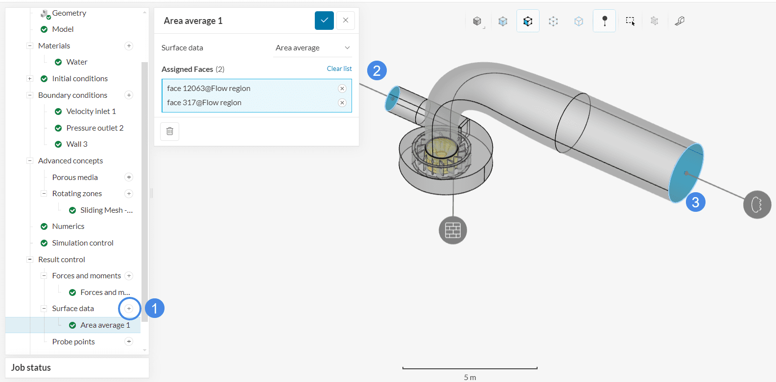
b. Area Average
For the second control, click on the ‘+ button’ next to Surface data. Create an ‘Area average’ control for the inlet and the outlet, as shown in Figure 18 below.
c. Pressure Difference
We can also get the pressure difference between the inlet and the outlet directly as follows:
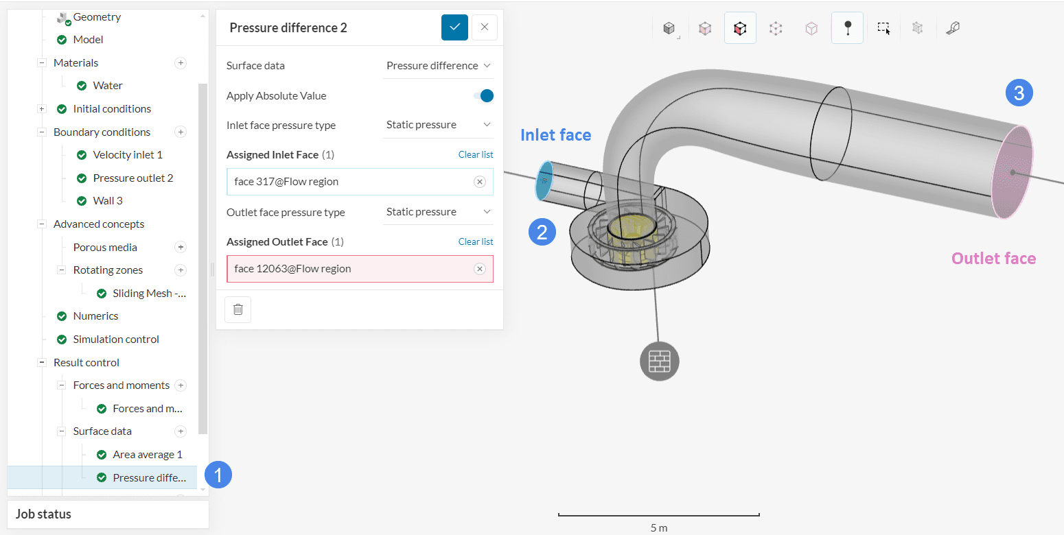
This comes handier when generating a pressure curve for multiple flow rates (parametric studies).
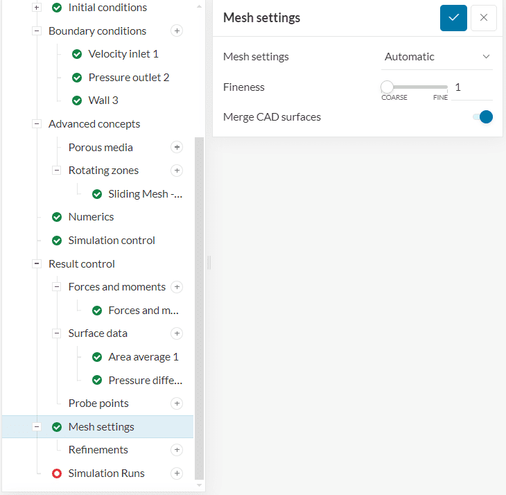
To create the mesh, we recommend using the Automatic mesh algorithm, which is a good choice in general as it is quite automated and delivers good results for most geometries.
In this tutorial, a mesh fineness level of 1 will be used. If you wish to undertake a mesh refinement study, you can increase the fineness of the mesh by sliding the mesh to higher refinement levels or using the region refinements.
Since this is a transient simulation, it is recommended to start with coarse mesh settings and gradually increase if required to save on core hours.
Did you know?
The automesher creates a body-fitted mesh which captures most regions of interest using physics based meshing.
If you are using a the manual mesher, you can learn how to set up different parameters in this Multi-purpose manual meshing documentation page.
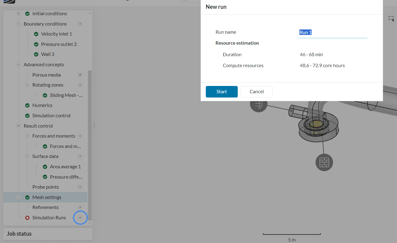
Now you can start the simulation. Click on the ‘+’ icon next to Simulation runs. This opens up a dialogue box where you can name your run and ‘Start’ the simulation.
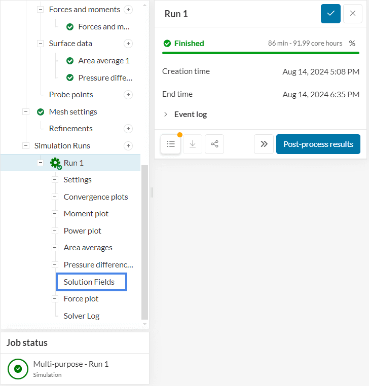
While the results are being calculated, you can already have a look at the intermediate results in the post-processor by clicking on ‘Solution Fields’ or ‘Post-process results’. They are being updated in real-time!
Depending on the instance chosen by the machine, it might take 1.5 to 4 hours for the simulation to finish.
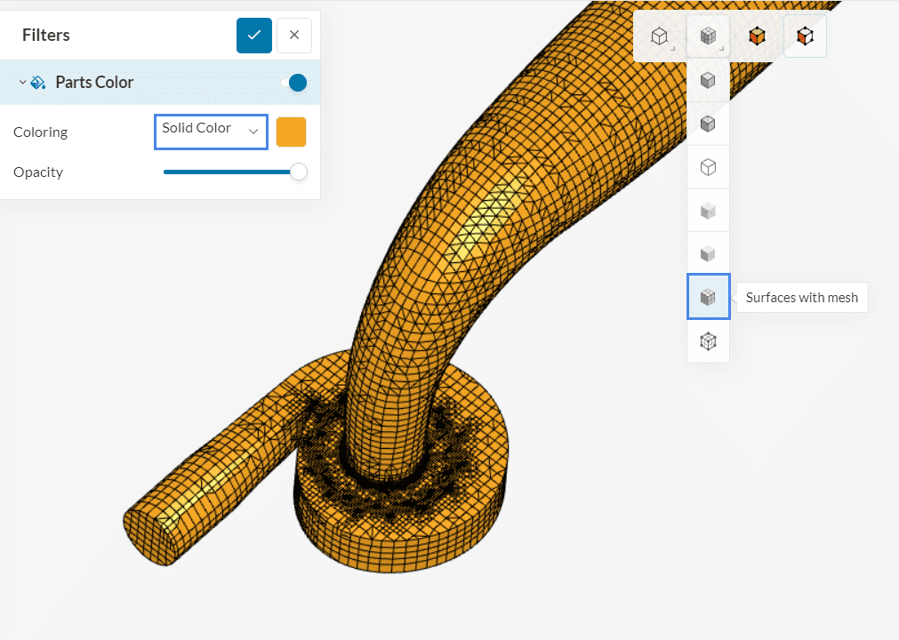
Once inside the post-processor, under the Parts Color filter change Coloring to any solid color of choice and then change the render mode to Surfaces with mesh to show opaque surfaces of the CAD model with the mesh grid.
You can use the cutting plane filter to see the inside of the mesh generated:
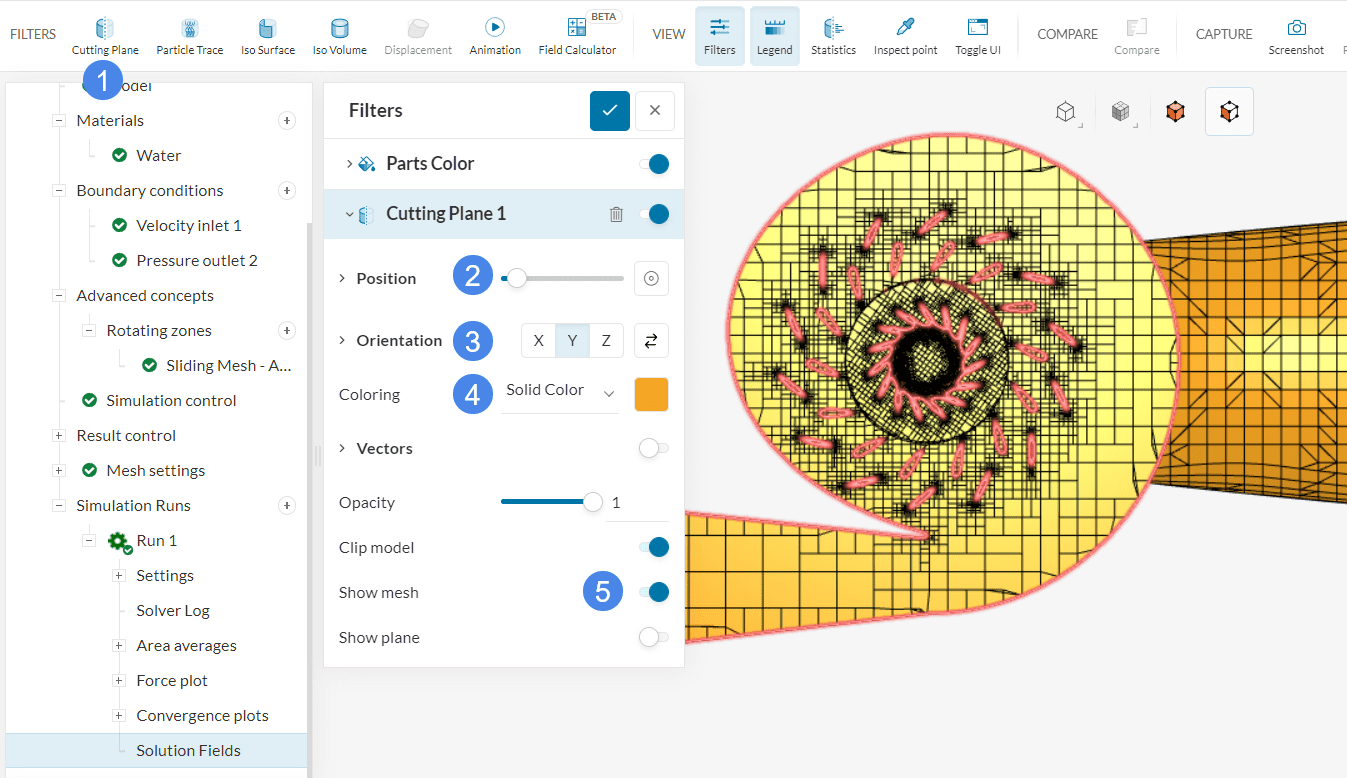
After a few seconds, you will see a clip showing the inside of your mesh. This mesh looks sufficient for this tutorial.
Did you know?
You can also select single faces of the geometry and hide them. This way, you can inspect inner surfaces.
One of the most important parameters to observe when evaluating the performance of a water turbine is how much the pressure drops after the water has flown through the turbine. You can calculate the pressure drop by subtracting the inlet pressure from the outlet pressure using area average plots or directly find the value of \(\delta\)p under Area Averages > Pressure difference.
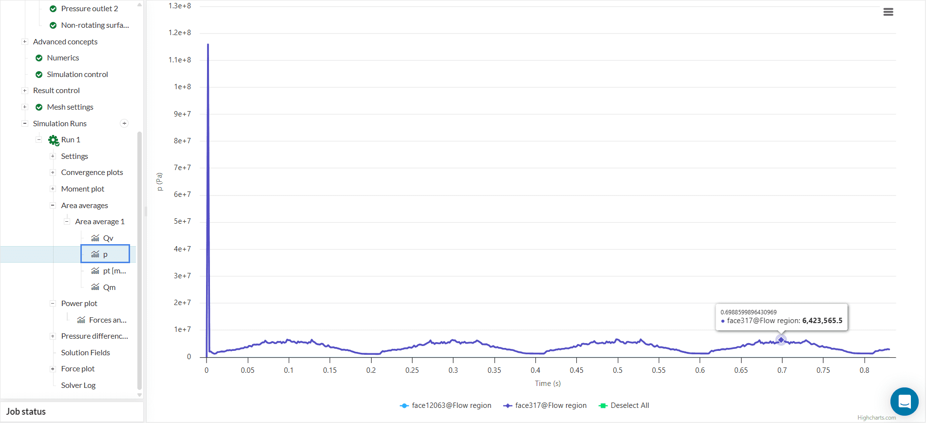
Figure 25 shows that the pressure variation is transient in nature. Calculate the average for these values, for example, from time step 0.6 to 0.8, which completes one wave of transience, which gives the pressure drop due to the turbine to be approximately 3.819 \(MPa\).
The Forces and moments results are of particular interest in a simulation with a turbine. The runner of our turbine was rotating around the y-axis. Hence, let’s inspect the resulting pressure forces and the torque generated around said axis:
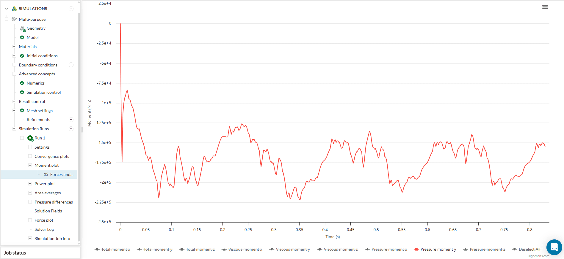
The resulting torque on the blades is given by the sum of all the moments around the rotation axis y.
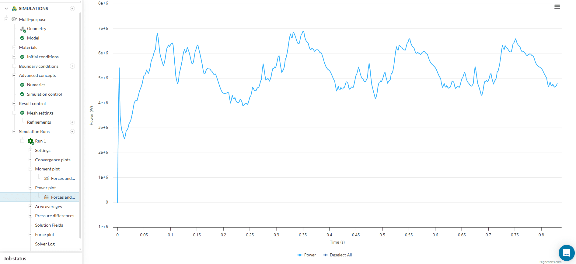
In this simulation, the average power output from the power plot comes out to be 5441.74 \(kW\). Hence, approximately 5442 \(kW\) of power is generated about the y-axis of this Francis turbine.
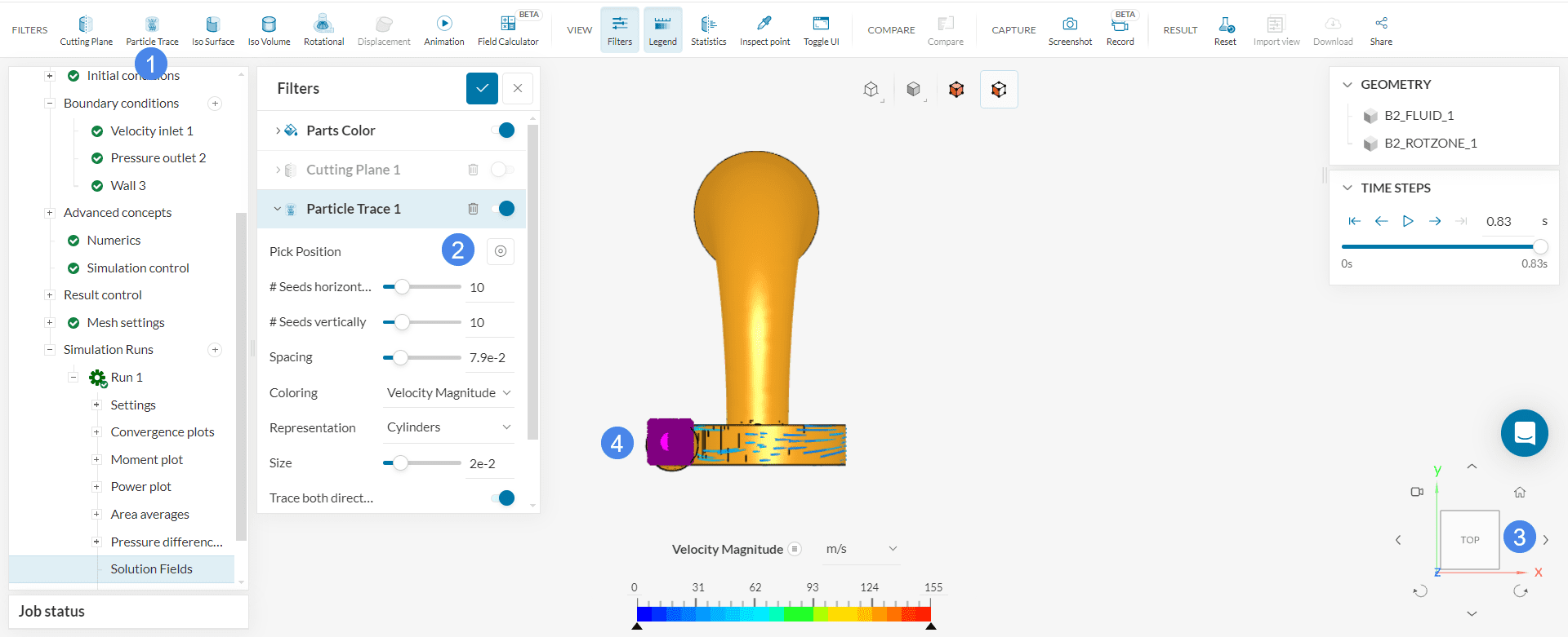
Streamlines can be a great tool to visualize flow patterns, especially in rotating machinery applications. Follow the steps below to show the flow streamlines inside the turbine:
Now repeat the process, but this time select the outlet as a seed face.
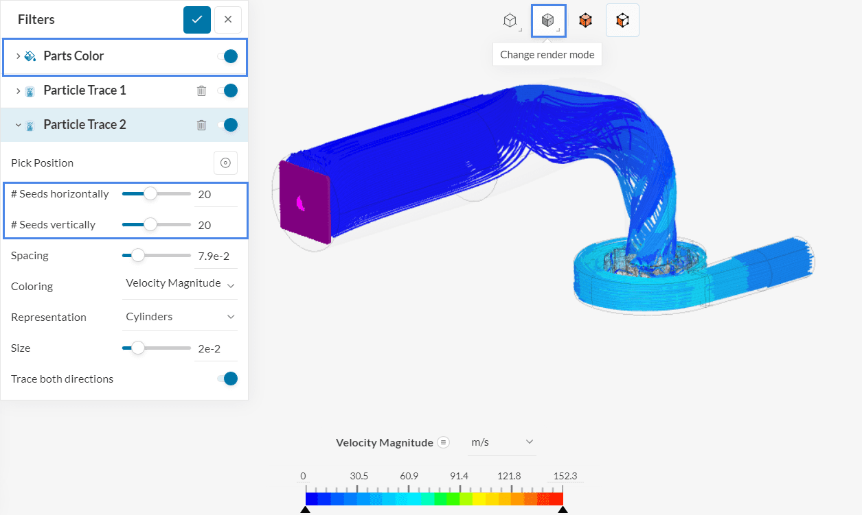
After the traces are created, you can adjust the render mode to ‘Translucent surfaces’ to give you a better view of the flow. We can see that the flow follows a circular motion in the outlet region due to the rotatory motion of the turbine.
To get more details on the flow behavior inside the turbine, use the Cutting plane filter.
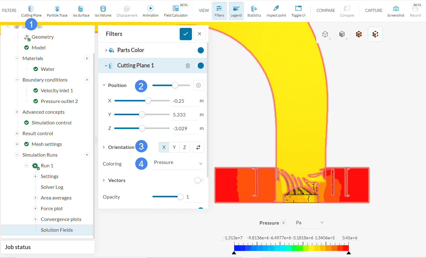
From Figure 30, you can see how the water pressure drops when flowing inside the turbine and decreases even more after flowing towards the outlet.
You can also see how the blades are affecting the flow by adjusting the position and orientation by following the instructions below:
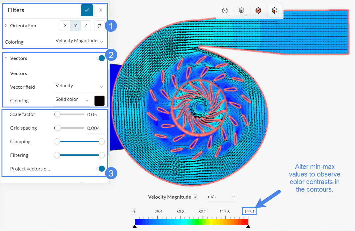
Any effect of the applied filters can be animated. Select ‘Animation’ from the top filter ribbon and click the play button under the Animation settings panel. Operate the animation commands as per your interests. Learn more.
In this view, you can get insights into how the blades and guide vanes are affecting the flow, allowing for optimizations in the design.
Analyze your results with the SimScale post-processor. Have a look at our post-processing guide to learn how to use the post-processor.
Note
If you have questions or suggestions, please reach out either via the forum or contact us directly.
Last updated: April 6th, 2026
We appreciate and value your feedback.
Sign up for SimScale
and start simulating now


