Tutorial: Fluid Flow through a Centrifugal Pump Using Multi-purpose Solver
This tutorial demonstrates how to use SimScale to run a centrifugal pump simulation using the Multi-purpose solver.
Overview
This tutorial teaches how to:
- Create a rotating region and extract flow volume for pump simulations.
- Set up and run an incompressible, steady state simulation.
- Assign saved selections.
- Assign boundary conditions, material, and other properties to the simulation.
- Mesh with the automatic meshing algorithm in Multi-purpose.
We are following the typical SimScale workflow:
- Prepare the CAD model for the simulation
- Set up the simulation
- Create a mesh
- Run the simulation and analyze results
1. Prepare the CAD Model and Select the Analysis Type
To begin, click the button below. It will copy the tutorial project containing the geometry into your Workbench.
The following picture demonstrates the original geometry that should be visible after importing the tutorial project.
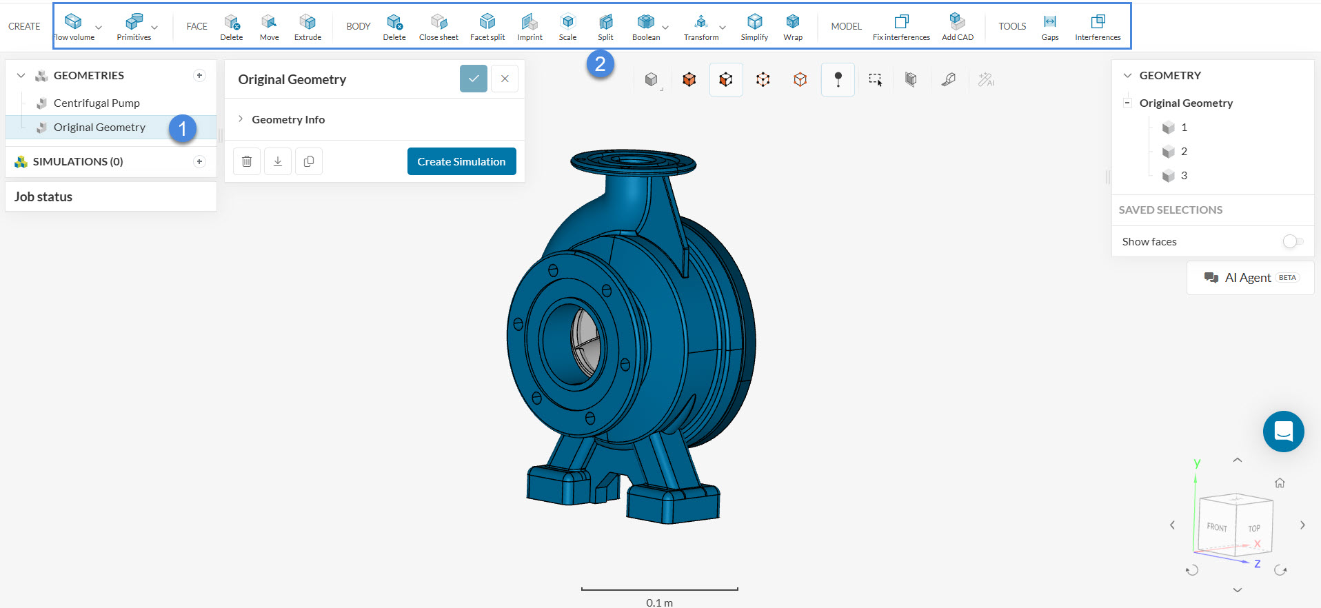
1.1 Geometry Preparation
Before starting to work using SimScale’s fluid simulator analysis with rotation, we need to make sure to prepare the CAD model to be compatible with this kind of analysis. This tutorial project contains two geometries, shown in the picture below:
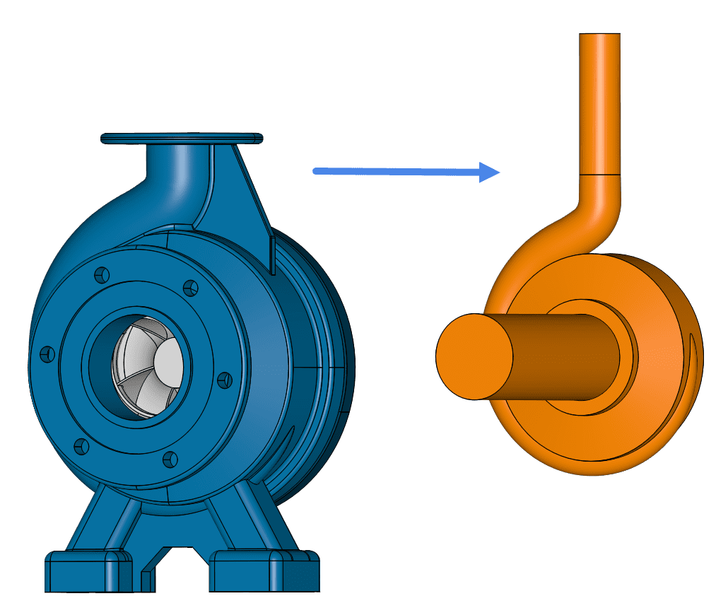
The first one (Original Geometry) consists of the actual pump and its blades. It still requires some preparation before it’s ready to use for CFD simulations. We’ll be using the second geometry already prepared for the simulation. If we needed to make modifications or to create the flow region ourselves, we’d need to use the CAD environment. To modify a CAD model, simply select the geometry from the list—the available CAD operations will then appear in the top toolbar. You can either work directly on the original model or create a duplicate and apply your changes to the copy.
What we need for a CFD simulation is the second geometry (Centrifugal Pump). It contains the flow region, as well as a volume representing the rotating zone. The steps to make the original geometry CFD-ready are fully described in the following article:
1.2 Create the Simulation
Make sure the Centrifugal Pump geometry is selected for this simulation project:
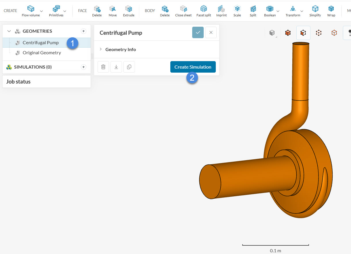
After hitting on ‘Create Simulation’, you will have several simulation types to choose from:
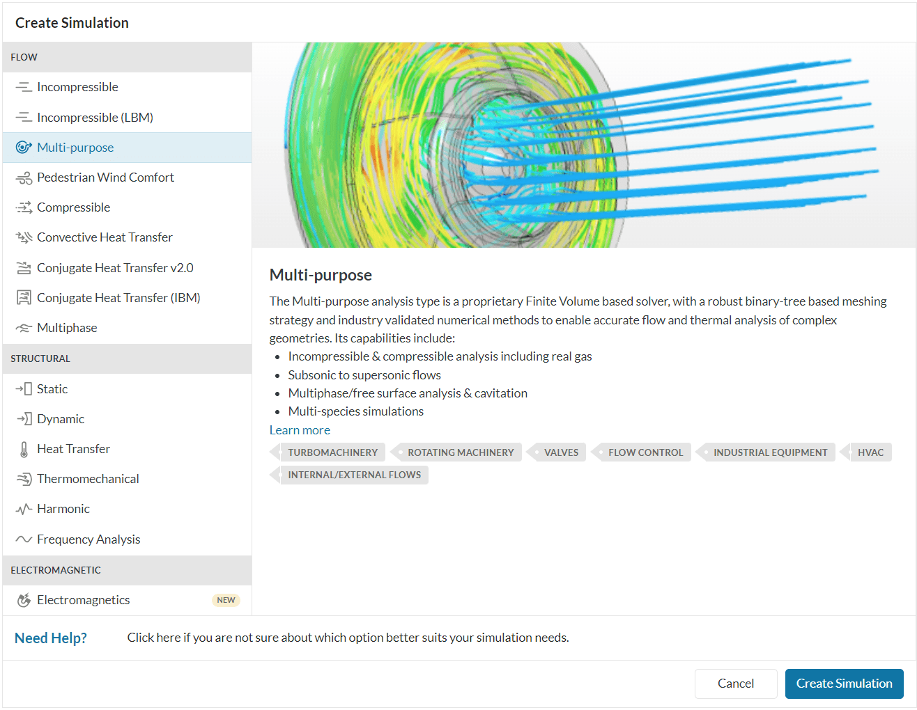
Choose ‘Multi-purpose’ as the analysis type and ‘Create Simulation‘.
At this point, the simulation tree will be visible in the left-hand side panel. To run the simulation, it’s necessary to configure the simulation tree entries.
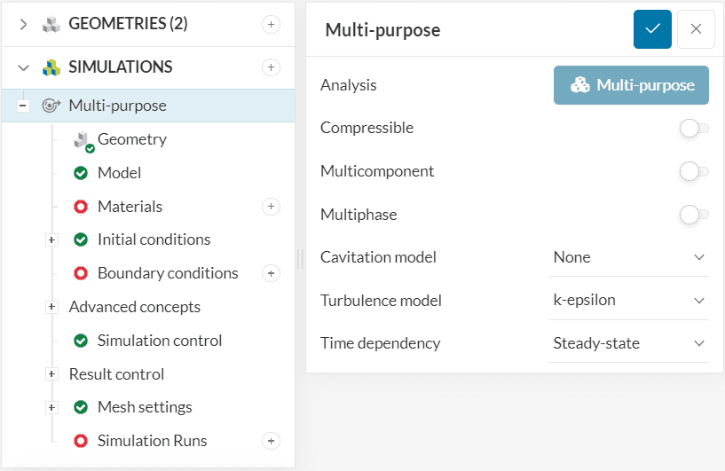
The global simulation settings remain as default, as in the figure above. With a Steady-state analysis, we will obtain the equilibrium state of the system, when the flow field no longer changes with time.
Did you know?
Within the pump blades, the flow experiences separation which is effectively captured by the k-epsilon turbulence model.
2. Pre-Processing: Setting up the Simulation
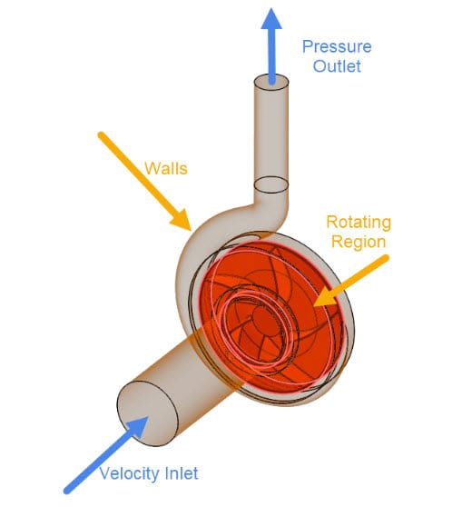
As an overview of the physics, the following picture shows the boundary conditions used in this project:
Did you know?
Velocity Inlet and Pressure Outlet is a very common combination used in CFD simulations as it often results in good stability. This combination permits flow to adjust aiming to assure mass continuity.
2.1 Define a Material
This simulation will use water as a material. Therefore click on the ‘+ button’ next to Materials. Doing this opens the SimScale fluid simulator material library as shown in the figure below:
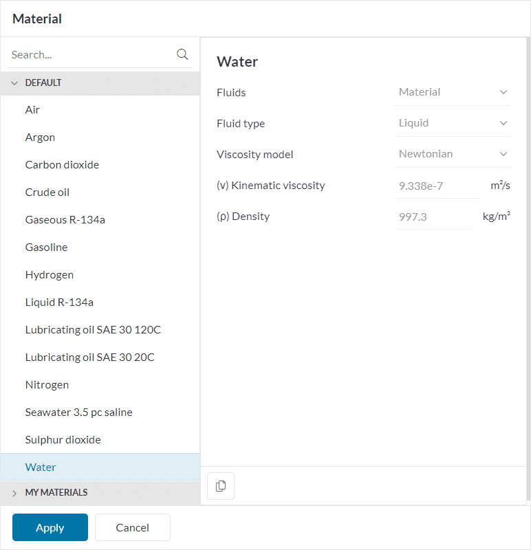
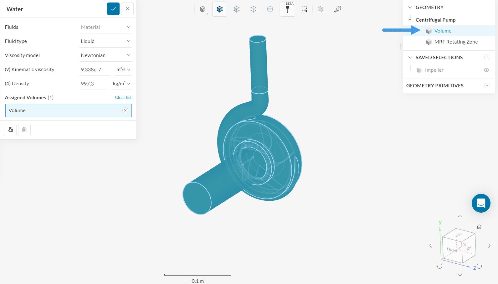
Select ‘Water’ and click ‘Apply’. A window opens up with the water properties. Keep the default values and assign them to the ‘Volume’ that represents the flow region.
Assigning Gravity
Note that there is a section on Model where the gravitational acceleration can be specified. This is useful for cases where gravity plays an important role. For the present tutorial, we will leave it to the default value of 0.
2.2 Assign the Boundary Conditions
In the next step, boundary conditions need to be assigned as in Figure 10. We have a velocity inlet, a pressure outlet, walls, and a rotating zone.
a. Velocity Inlet
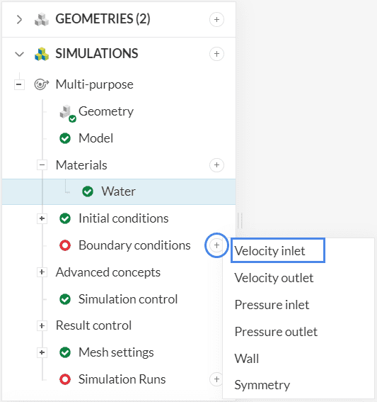
After hitting the ‘+ button’ next to Boundary conditions, a drop-down menu will appear, where one can choose between different boundary conditions.
After selecting ‘Velocity inlet’, you can specify the velocity configuration and assign the inlet face. Please proceed as follows:
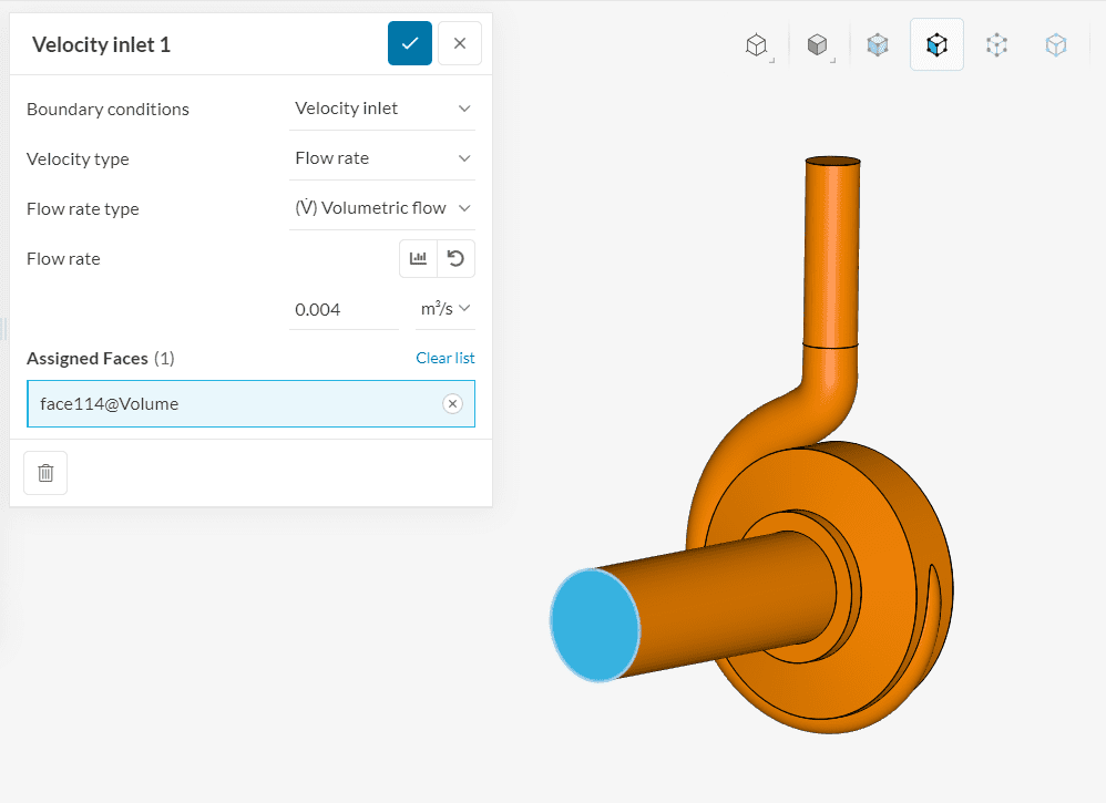
With these settings, a volumetric flow rate of ‘0.004’ \(m^3/s\) enters the domain through the inlet.
Parametric study with multiple flow rates
Multi-purpose analysis type allows parametric studies with the velocity boundary condition. When you select Flow rate as the velocity type while assigning velocity to an inlet or outlet face then you can input multiple flowrates at once either directly or by uploading a file.
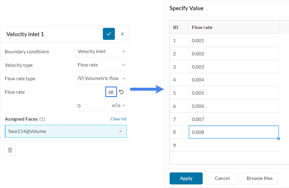
Enter multiple flowrates through the specify value icon as highlighted which opens up a new window to input the values in a table format. Hit ‘Apply’. Don’t forget to assign the inlet face.
This will help initiate multiple runs with different flow rates assigned at once in parallel giving the user a huge time advantage. In this tutorial, we encourage you to try this functionality.
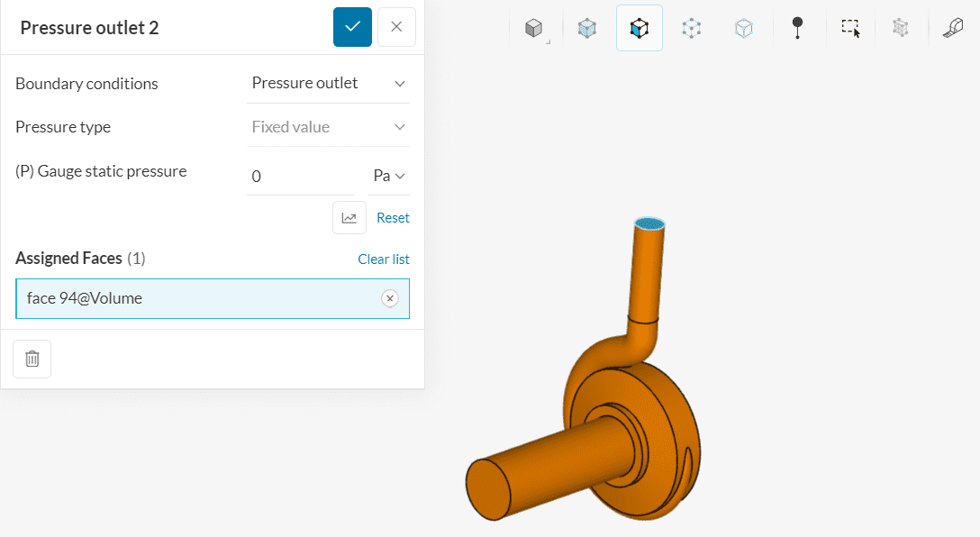
b. Pressure Outlet
Create a new boundary condition, this time a ‘Pressure outlet’ and select the outlet face. Make sure (P) Gauge Pressure is set to a fixed value of ‘0’ \(Pa\).
c. Walls
In Multi-purpose analysis, all the surfaces that act as walls are automatically treated likewise by the solver itself. Walls outside the rotating zone receive a no-slip condition and walls inside the rotating zone are treated as rotating walls unless you specifically pick the faces inside the rotating zone that you want to be static.
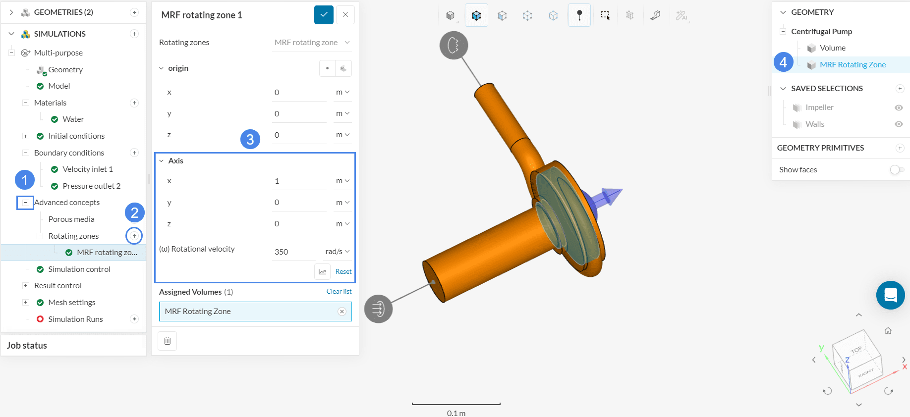
2.3 Advanced Concepts: Creating a Rotating Zone
In the simulation tree, please expand Advanced concepts. Click on the ‘+ button’ next to Rotating zones and select an ‘MRF Rotating Zone’. Define the MRF zone as shown:
Did you know?
Based on the initial input at the start of the simulation, Multi-purpose automatically assigns the rotating region as MRF or AMI zone. No additional input is required when setting up the rotating zone.
This article provides more information about the difference between MRF and AMI Rotating Zones.
2.4 Simulation Control
Don’t worry about the numerical settings for the Multi-purpose simulations, as their default values are optimized.
Open the simulation control settings and change the Number of iterations to ‘600’.
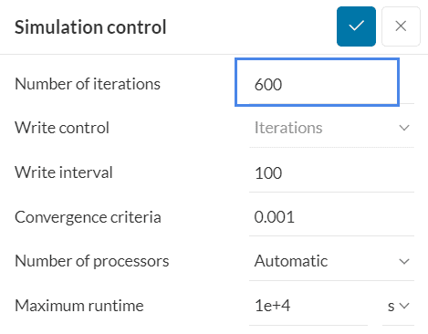
Keep the remaining settings as default. To know more about how to control the simulation read in detail here.
2.5 Result Control
Result control allows you to observe the convergence behavior at specific locations in the model during the calculation process. Hence, it is an important indicator of the simulation quality and the reliability of the results.
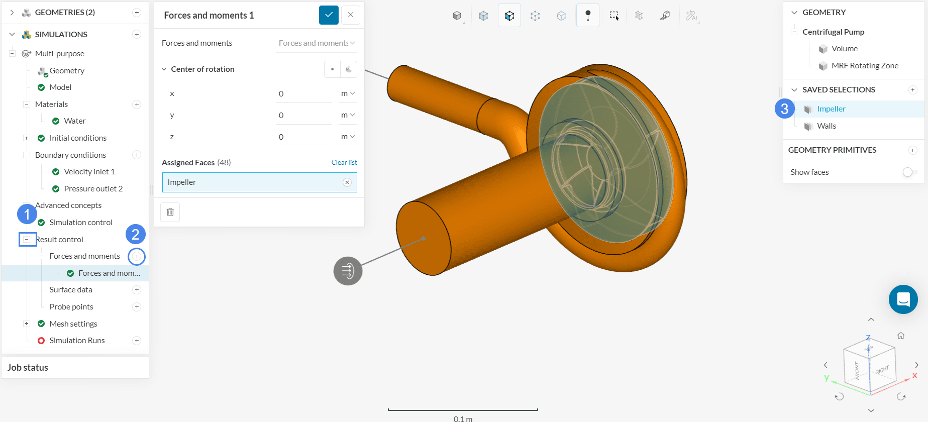
a. Forces and Moments
For this simulation, please set a ‘Forces and moments’ control to the impeller. To save time, there’s a pre-saved saved selection for the Impeller surfaces:
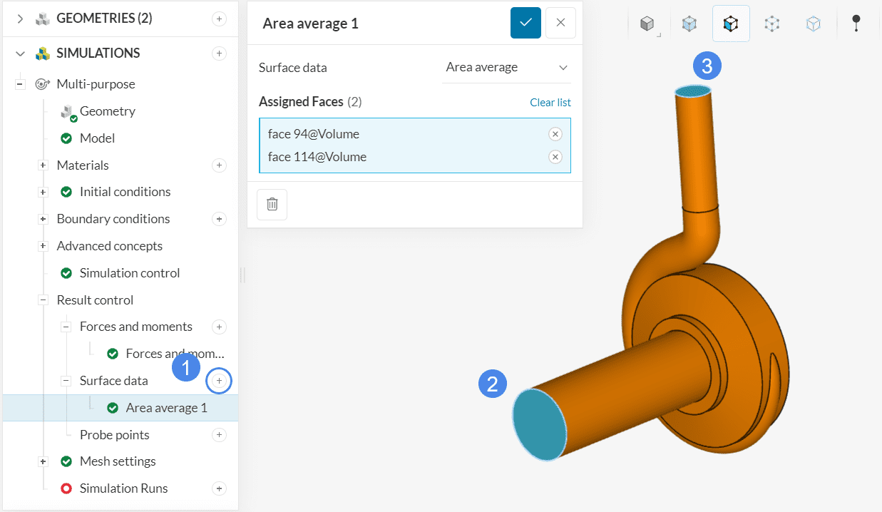
b. Area Average
Finally, click on the ‘+’ button next to Surface data. Create an ‘Area average’ for the inlet and the outlet:
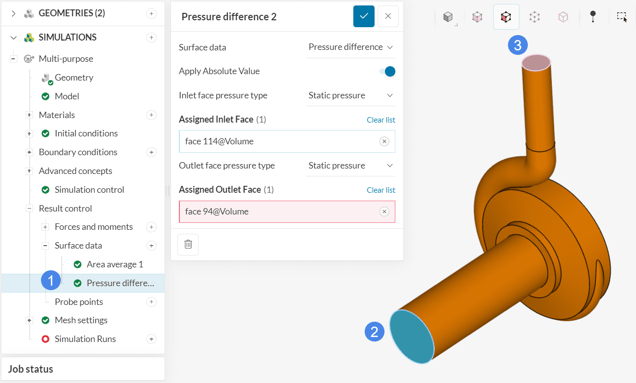
c. Pressure Difference
To get the pressure difference between the inlet and the outlet directly set up Pressure difference curves as well. This result control item creates a plot each for the different flow rates with respect to iterations and also creates a pressure curve for the turbine.
3. Mesh
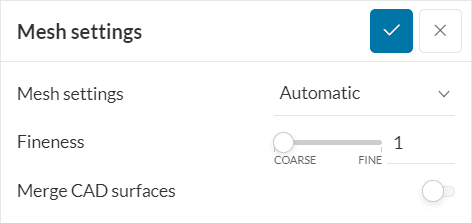
To create the mesh, we recommend using the Automatic mesh algorithm, which is a good choice in general as it is quite automated and delivers good results for most geometries.
In this tutorial, a mesh fineness level of 1 will be used for demonstration purposes. If you wish to undertake a mesh refinement study, you can increase the fineness of the mesh by sliding the mesh to higher refinement levels.
Did you know?
The automesher creates a body-fitted mesh which captures most regions of interest using physics based meshing.
If you are using a the manual mesher, you can learn how to set up different parameters in this Multi-purpose manual meshing documentation page.
4. Start the Simulation
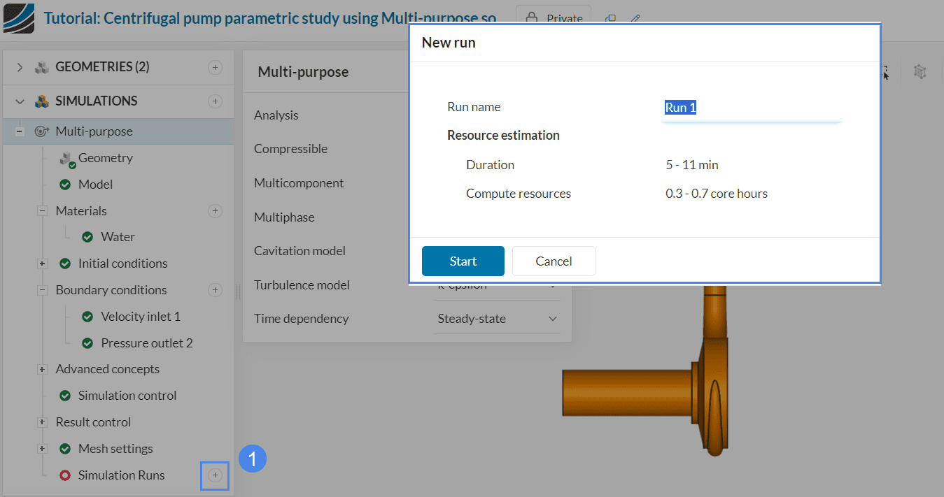
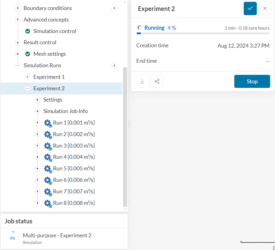
Now you can start the simulation. Click on the ‘+’ icon next to Simulation runs. This opens up a dialogue box where you can name your run and ‘Start’ the simulation.
While the results are being calculated you can already have a look at the intermediate results in the post-processor by clicking on ‘Solution Fields’. They are being updated in real-time!
It takes roughly 5-8 minutes for the simulation to finish.
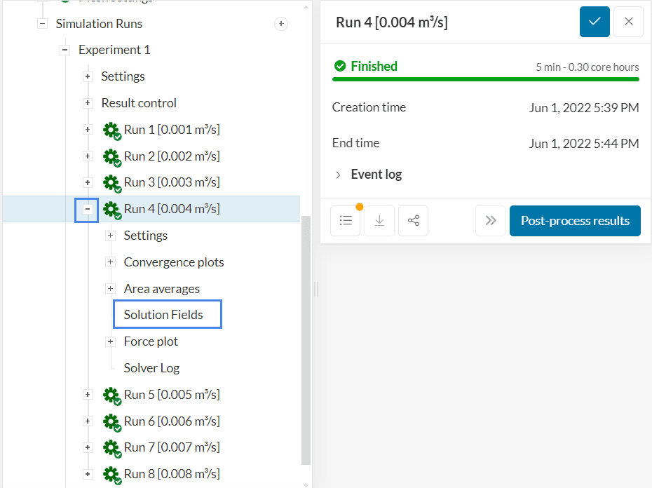
SimScale has a built-in post-processing environment, which can be accessed by clicking on ‘Solution Fields’, as in Figure 25:
Did you know?
With SimScale, it’s easy to get the pump curve for your geometry. You can run multiple simulations in parallel, only changing the flow rate (in the velocity inlet boundary condition).
For more information about pump curves, please check out this blog post.
5. Post-Processing
5.1 Visualizing the Mesh
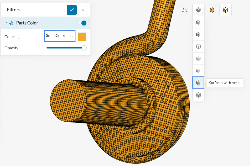
Once inside the post-processor, under the Parts Color filter change Coloring to any solid color of choice and then change the render mode to Surfaces with mesh to show opaque surfaces of the CAD model with the mesh grid.
You can use the cutting plane filter to see the inside of the mesh generated:
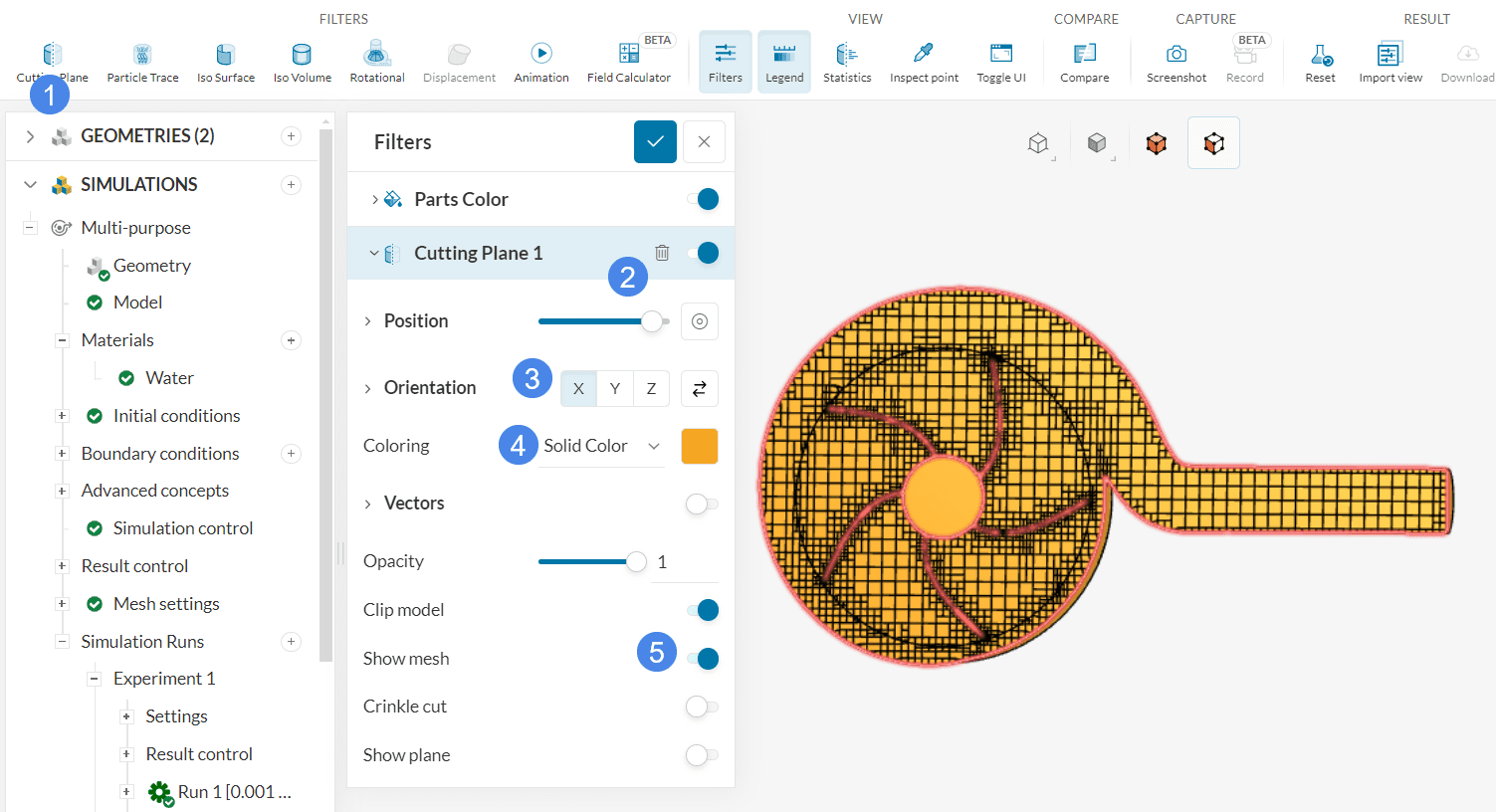
- Hit the ‘Cutting Plane’ filter from the top ribbon.
- Adjust the position until it cuts the rotor.
- Adjust the orientation to X axis.
- Change the Coloring to some contrasting solid color.
- Toggle on Show mesh so that the mesh can be visible.
After a few seconds, you will see a clip showing the inside of your mesh. This mesh looks sufficient for this tutorial.
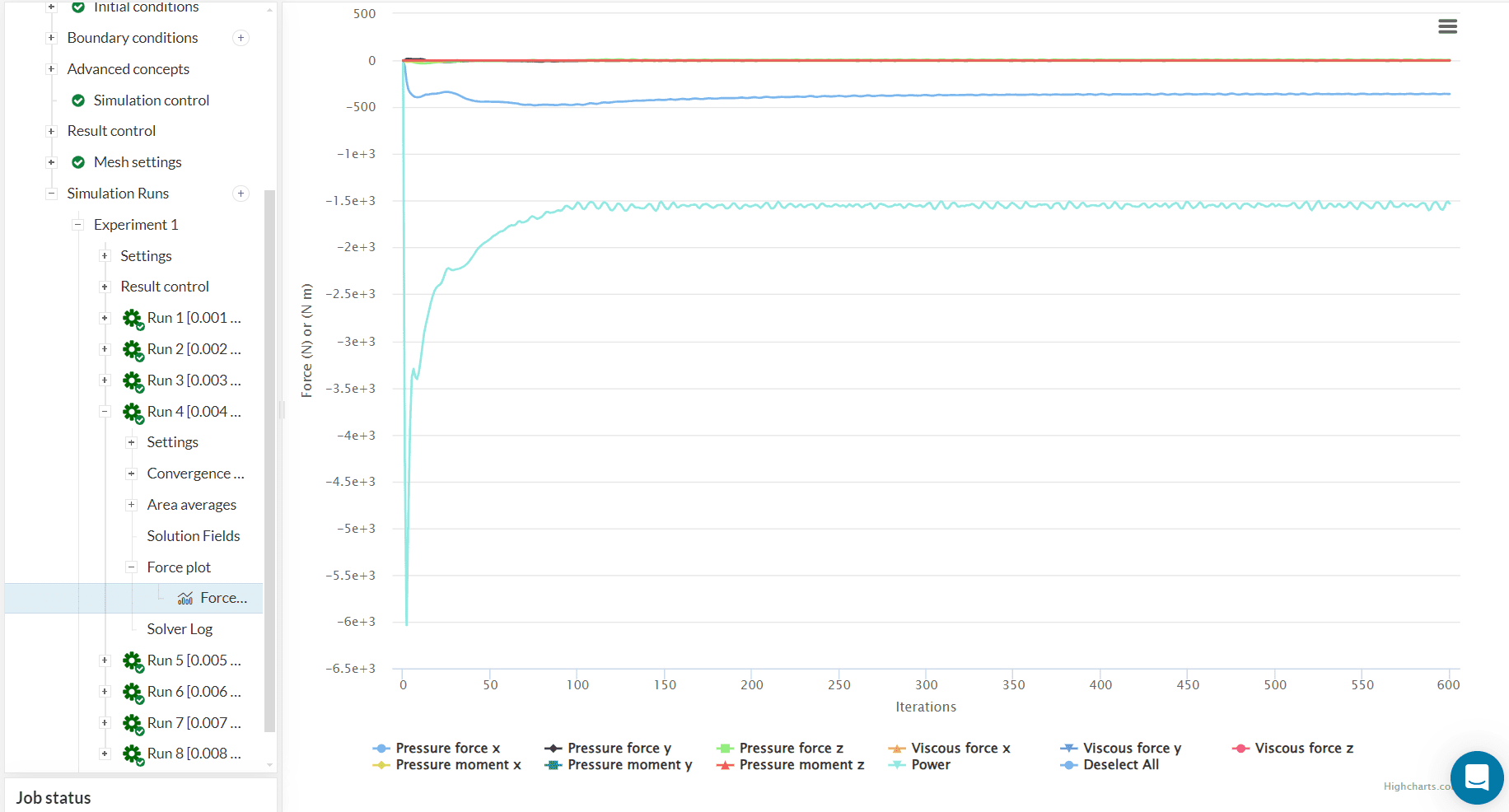
5.2 Convergence Behavior
With the previously set result controls, it’s possible to assess convergence. As the iterations go on, key parameters are expected to stop changing. At this point, the simulation is considered converged.
So what are the key parameters? For a centrifugal pump simulation, the velocity at the outlet, the pressure at the inlet, and forces onto the impeller are parameters of interest. For example, let’s have a look at the forces and moments plot:
5.3 Performance Curve
Since we ran multiple simulations in parallel, the pressure difference \(\Delta p\) is plotted with respect to all flowrates. This is available under Result control>Area averages:
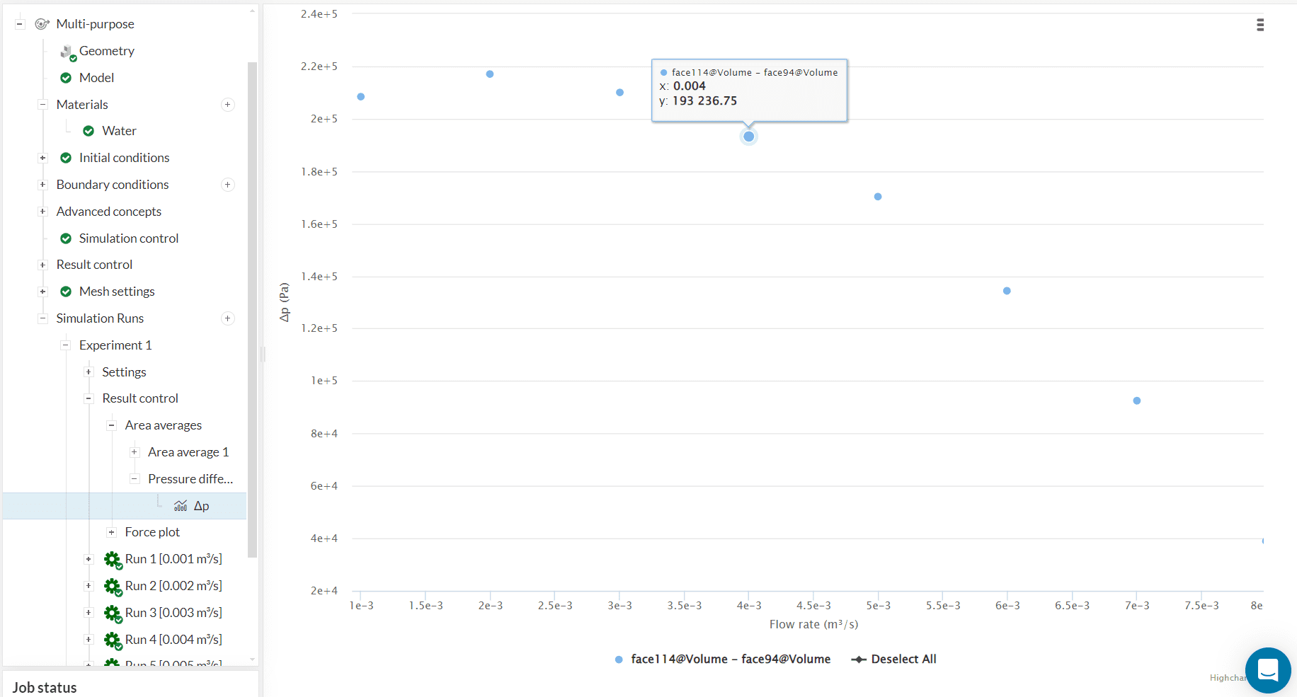
A Pump performance curve defines the range of possible operating conditions for the pump. Pump curves can tell about a pump’s ability to produce flow under a certain pressure head, as well as its efficiency and braking horsepower. Pump curves are essential for optimal pump selection as well as reliable and efficient operation.
5.4 Pressure
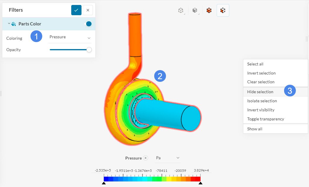
- Under Parts Color, make sure that the Coloring is ‘Pressure’. This way, the pressure levels are displayed on the boundaries.
- To make the blades visible, you can select the outer faces by clicking on them.
- Once you select the faces, right-click on the viewer and choose ‘Hide selection’.
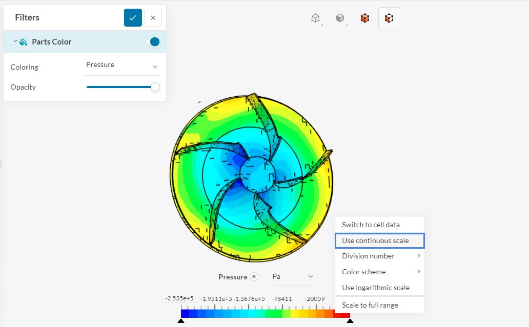
After hiding the first set of faces, you may have to hide more internal faces before the blades are fully visible. At this stage, right-click on the legend and select ‘Use continuous scale’ to make the color scheme smoother:
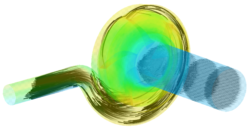
5.5 Velocity Vectors
To get a better understanding of what is going on inside the pump, proceed to add a ‘Cutting Plane’ filter:
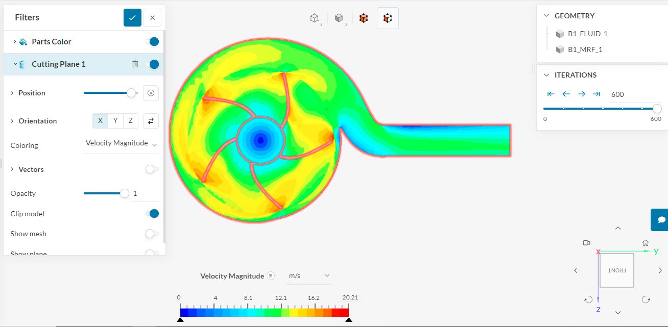
- Create a ‘Cutting Plane’ filter by using the top ribbon.
- Adjust the Position coordinates of the cutting plane to ‘0, 0, 0’. Furthermore, make sure that the Orientation is ‘X’ and the Coloring is ‘Velocity Magnitude’.
- Ensure Clip model is toggled on.
You can also toggle on Vectors to check the flow direction of the field in different areas:
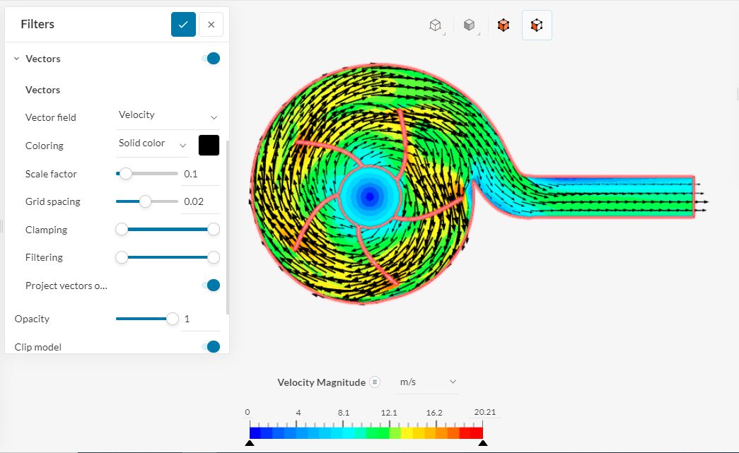
- Change the Coloring to ‘Solid color’, and select the black color from the available options.
- Then set the Scale factor to ‘0.1’ and the Grid Spacing to ‘0.02’.
- Activate the ‘Project vectors onto plane’ option.
Near the edges of the blades, the acceleration of the flow can be distinguished due to the representation with a warmer color compared to its surroundings. Other configurations for the cutting plane will give you additional information. For instance, you can change the Orientation to ‘Y’
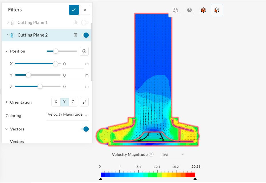
With this configuration, you can observe the flow pattern around the blades from a different perspective.
Analyze your results with the SimScale post-processor. Have a look at our post-processing guide to learn how to use the post-processor.
Note
If you have questions or suggestions, please reach out either via the forum or contact us directly.
Last updated: April 6th, 2026
Did this article solve your issue?
How can we do better?
We appreciate and value your feedback.


