Documentation
In this tutorial, you will learn to quickly set up a basic structural simulation of a connecting rod and conduct stress analysis using SimScale.
This tutorial demonstrates the process of setting up and executing a linear static analysis on a wheel loader arm using SimScale. The steps covered follow the standard SimScale simulation workflow and include:
Objectives
Throughout the tutorial, the following tasks will be performed:
Begin by selecting the button below. This action copies the tutorial project, including the geometry, into the SimScale Workbench for further setup and simulation.
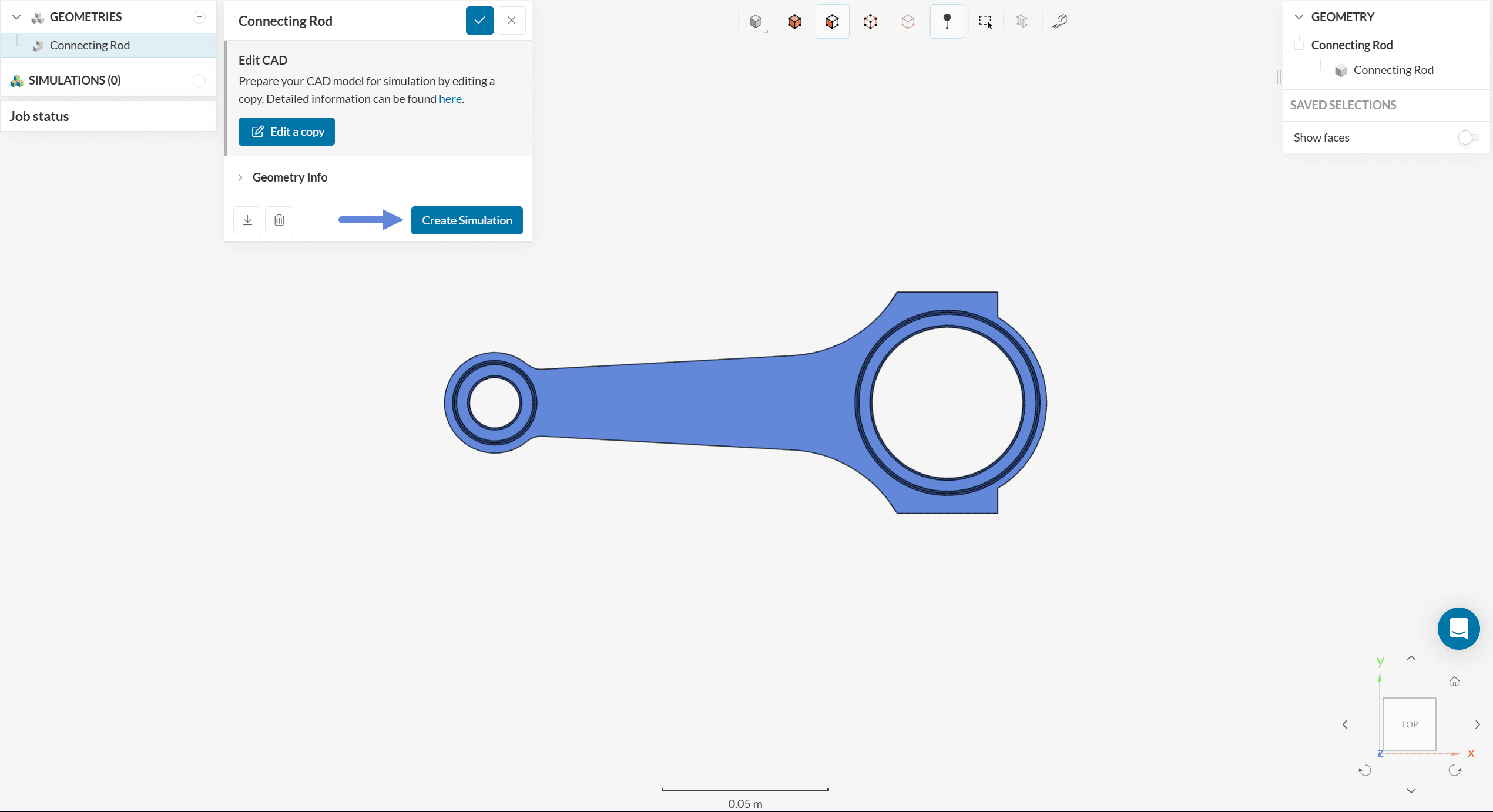
To begin the simulation setup, use the ‘Create Simulation’ button located in the geometry dialog box. This opens the simulation creation panel where analysis types can be selected.
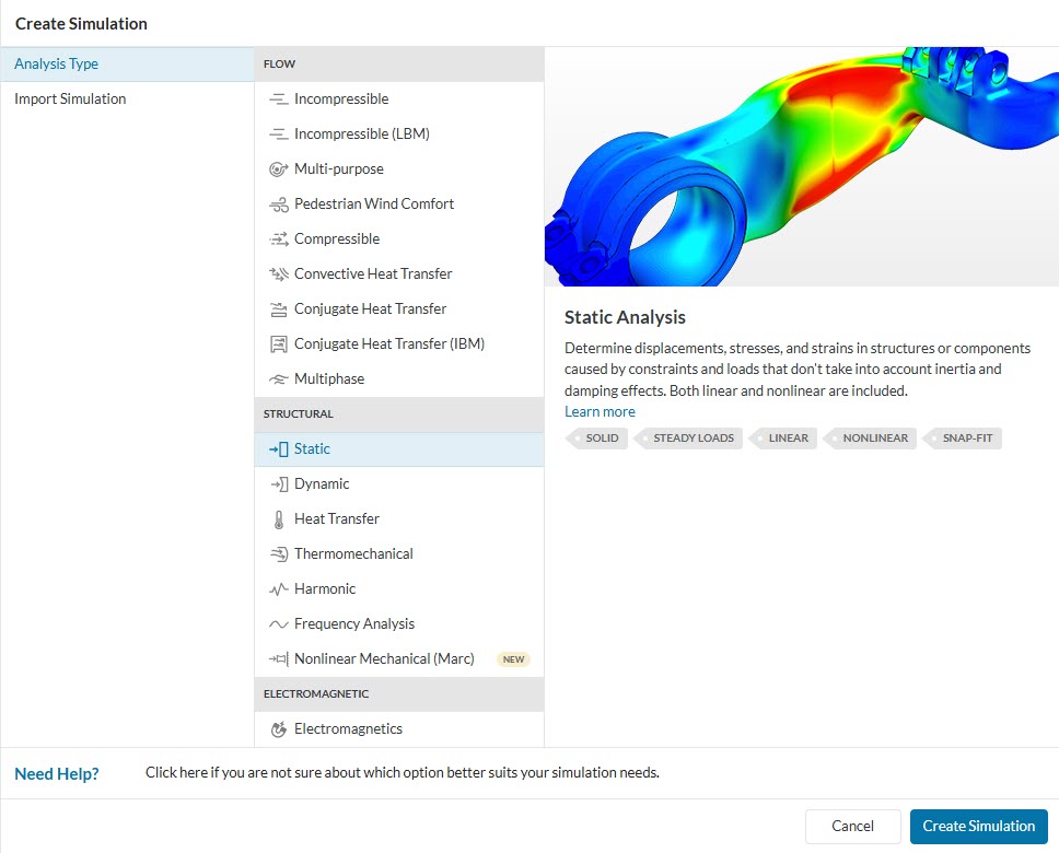
At this stage, the simulation type selection panel appears, allowing the choice of the desired analysis type from the available options. Select the ‘Static’ analysis type for this simulation.
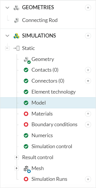
The platform then displays the simulation tree, which lists all settings that must be defined before running the analysis.
A new Simulation tree will automatically be generated on the left side of your Workbench, containing all parameters and settings required to start the simulation.
Before running the simulation, define the following key settings:
To define and modify the direction of gravity, click on ‘Model’.
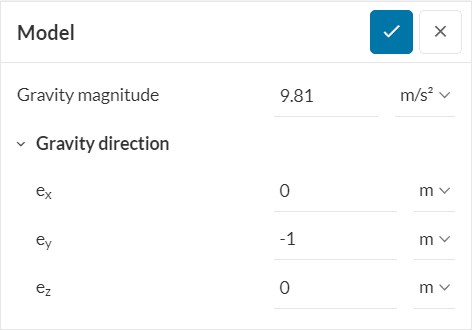
This will open up the settings panel for Model. In this case, gravity is acting in the negative y-direction. Add ‘9.81’ m/s as the magnitude and ey as ‘-1’ to indicate gravity in the negative-y direction.
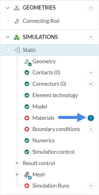
To assign a material to your model, click on the ‘+’ button next to Materials in the simulation tree.
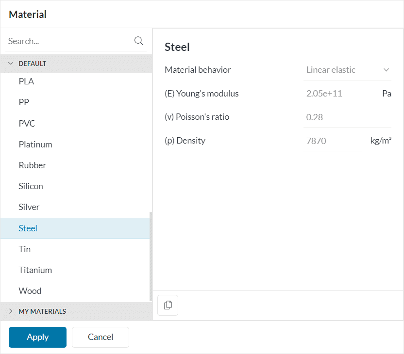
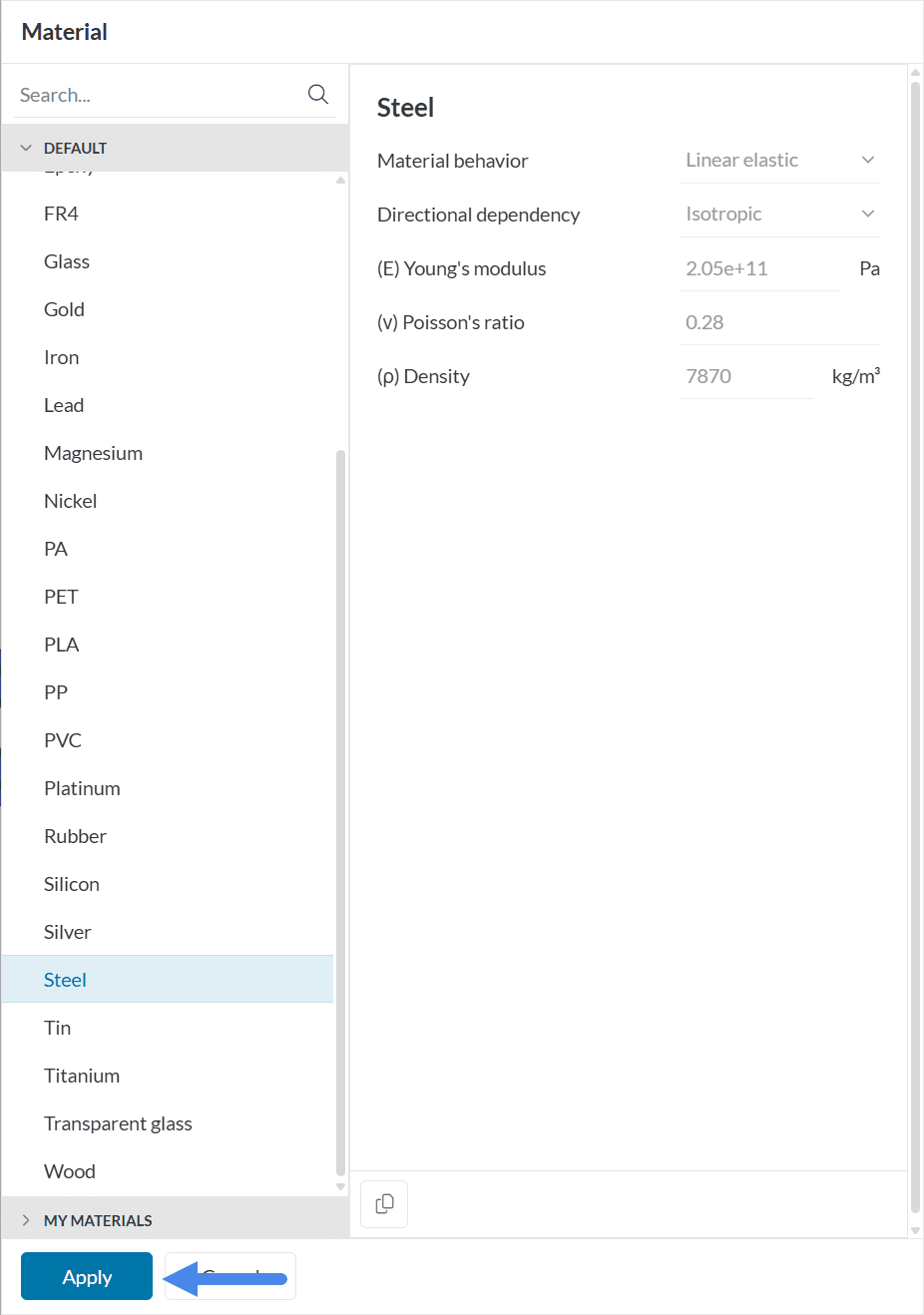
The Material library will open containing pre-defined materials. Scroll down to select ‘Steel’ and click ‘Apply’.
The material will automatically be assigned to the connecting rod.
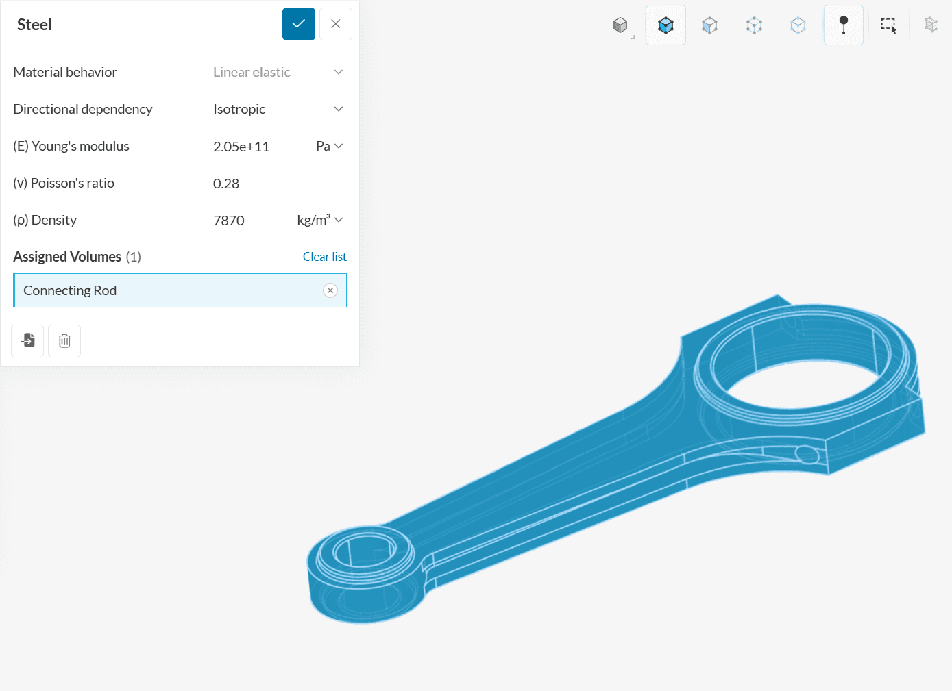
Note
The color blue indicates that the material has been assigned.
Two boundary conditions, pressure (load) and fixed support, need to be assigned to the connecting rod.
A. Pressure
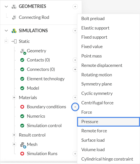
To create a new boundary condition, click on the ‘+’ button next to Boundary conditions in the simulation tree. Select ‘Pressure’ from the list.
Set the pressure value to ‘200’ bar. You can change the units from the dropdown by selecting ‘bar’ as the unit of pressure (see Figure 10).
Now select the faces on which the pressure should act. In the viewer, select the four inner faces inside the smaller opening of the rod.
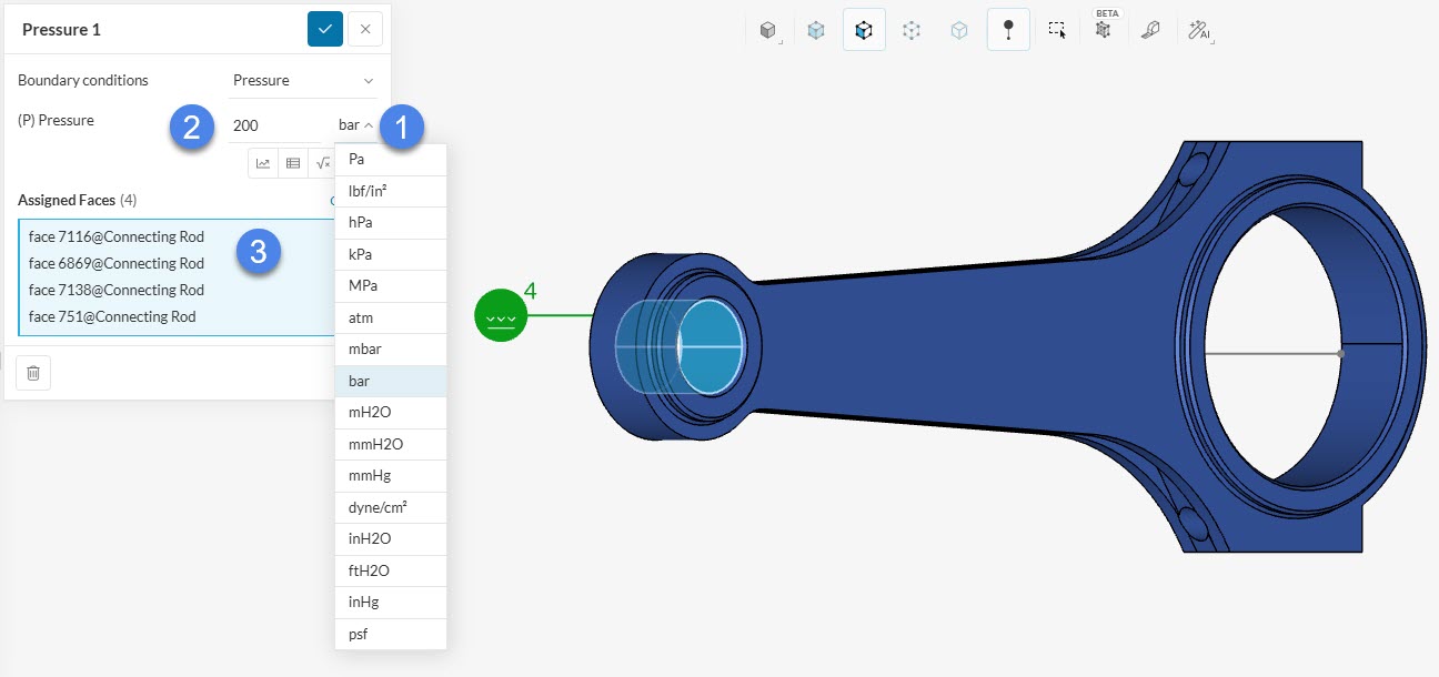
Note
The color turns blue, indicating that they will be assigned to the current boundary condition.
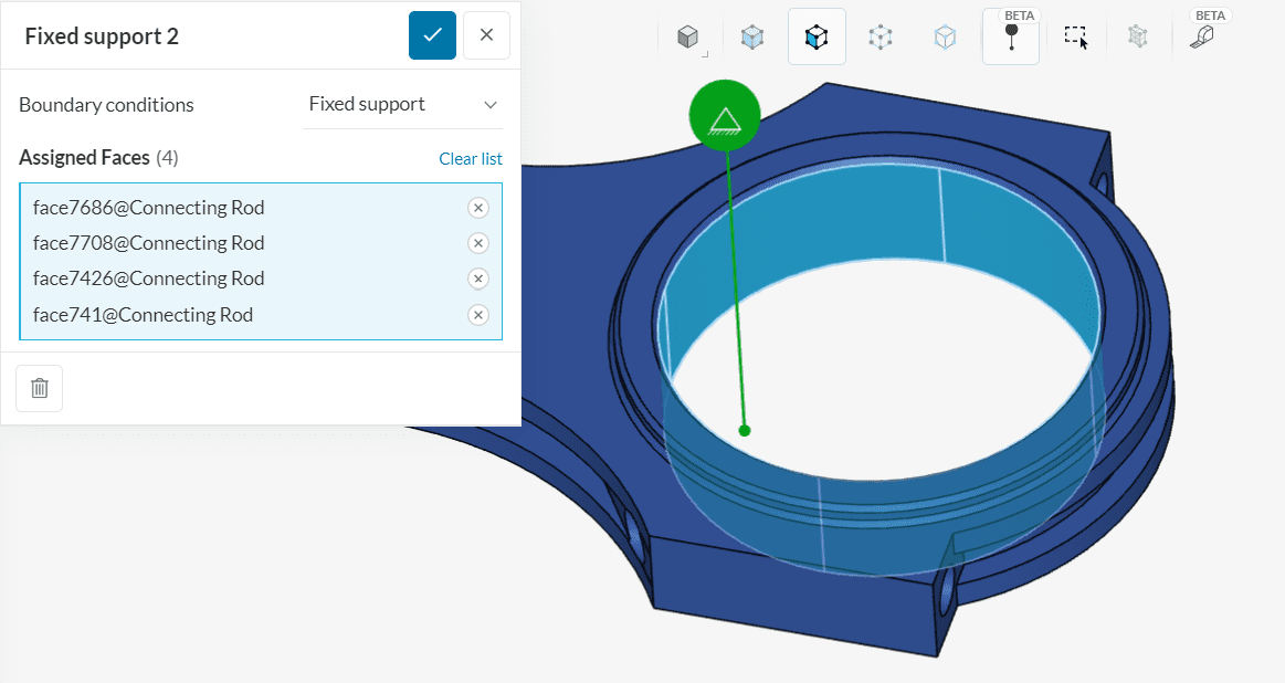
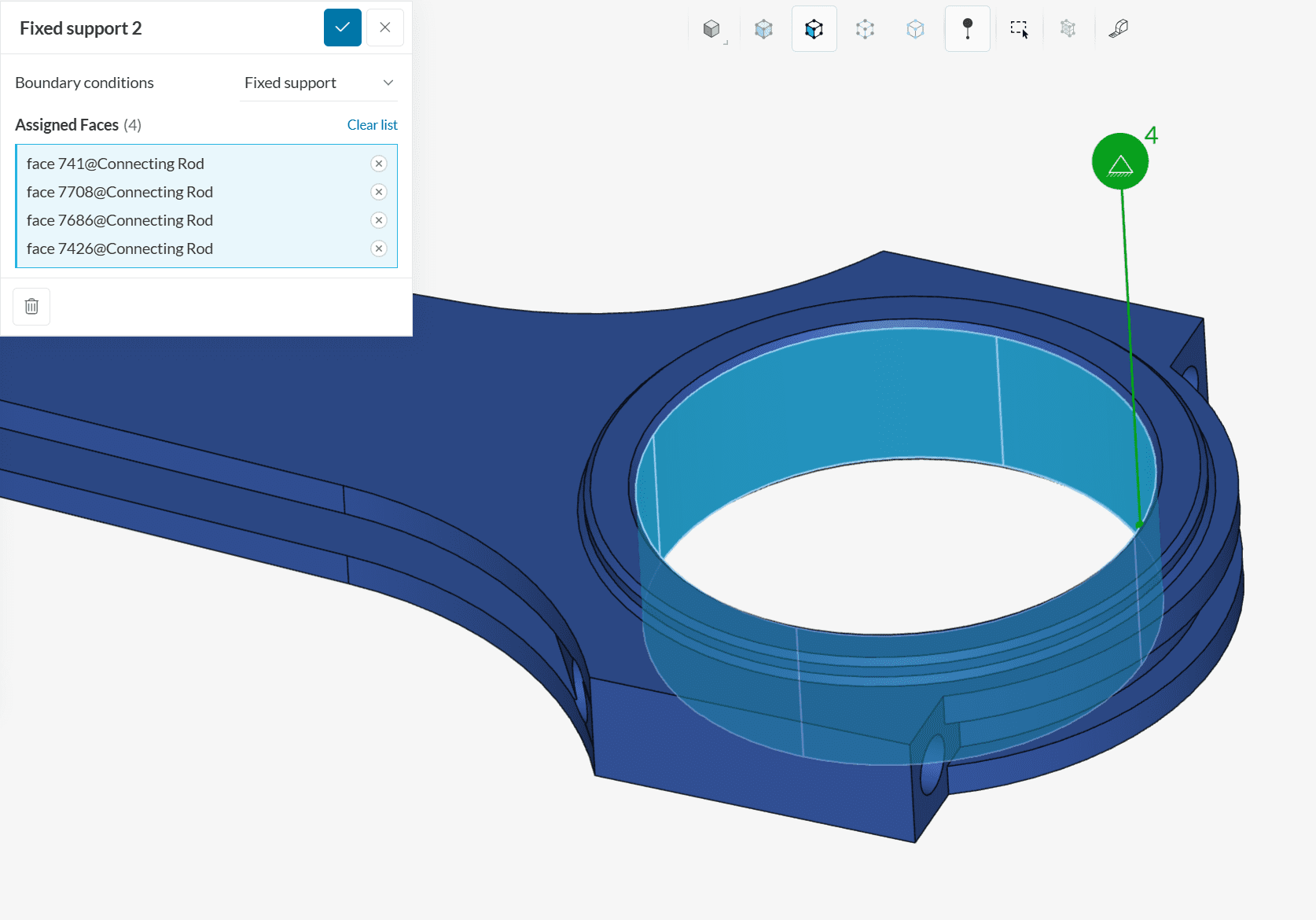
B. Fixed Support
Repeat the process and add another boundary condition by clicking on the ‘+’ button next to Boundary conditions. Select ‘Fixed Support’. Assign all the inner faces at the larger end of the connecting rod in the viewer.
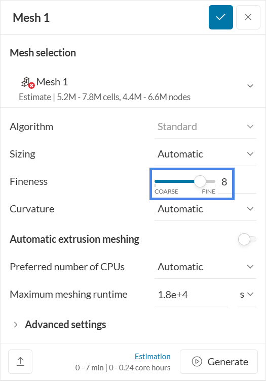
To generate the mesh, use the ‘Standard’ meshing algorithm, which is automated and typically provides good results for most geometries. For this simulation, the only change to be applied to the default settings is changing the fineness level to ‘8’ – and the mesh can be obtained by clicking the ‘Generate’ button. In linear static simulations, SimScale automatically creates second-order meshes, which enhance the accuracy of the analysis.
Why 2nd Order Elements?
Second-order elements are generally recommended for static analyses due to their improved accuracy in capturing deformation and stress gradients. For more details, refer to the article:
Which type of finite element should I use?
The mesh order can be specified under the Element Technology tab in the simulation tree. More information is available here:
Element Technology
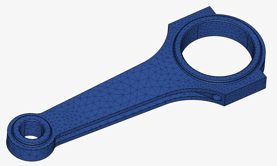
The resulting mesh appears as shown below, illustrating the geometry discretized with second-order elements and a fineness level of 8.
Related Meshing Knowledge Base Articles
For further guidance on meshing techniques and best practices, consider reviewing the following knowledge base articles:
Now you are ready to start your simulation run. The Numerics and Simulation Control settings are set by default and do not have to be changed for this simulation.
Create a simulation run by clicking on the ‘+’ button next to Simulation Runs in the simulation tree. In the window that appears, click ‘Start’:
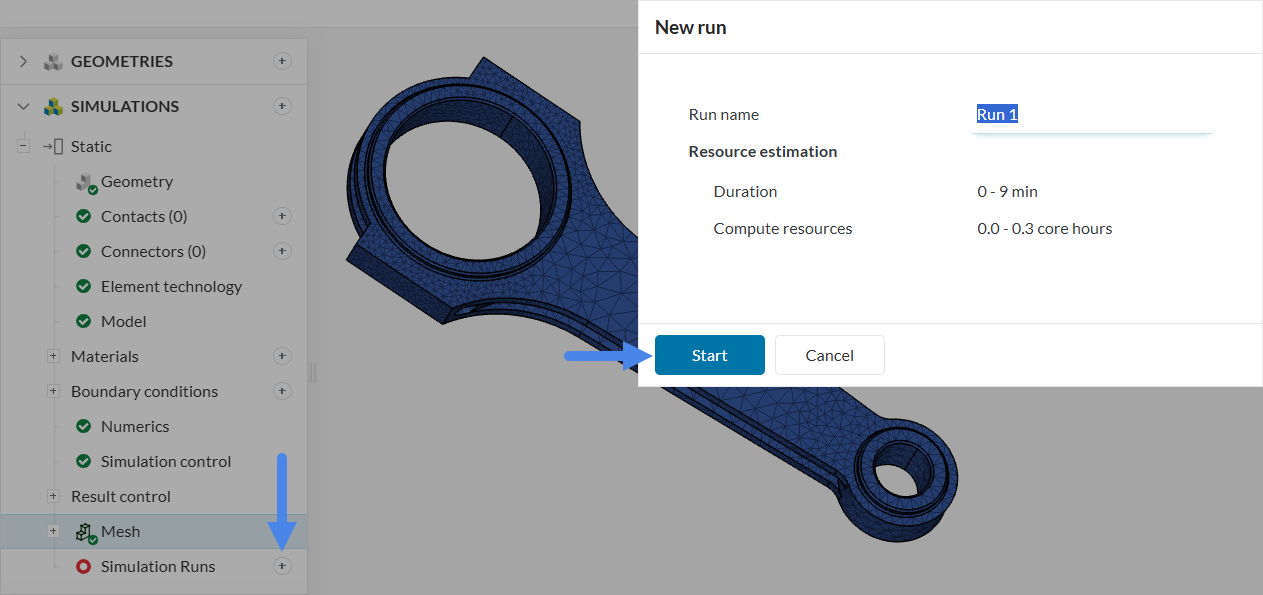
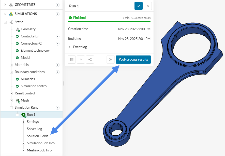
A dialog box will appear stating the estimated amount of resource consumption. Click ‘Start’ in the New run dialog box to start the simulation run. With this workflow, the mesh will be generated and after that the simulation starts right automatically. Once the simulation run is finished, its status will be changed to Finished in the run settings panel.
To access the post-processor you can click ‘Post-process results’ or ‘Solution fields’ under your run to load the results in the post-processor.
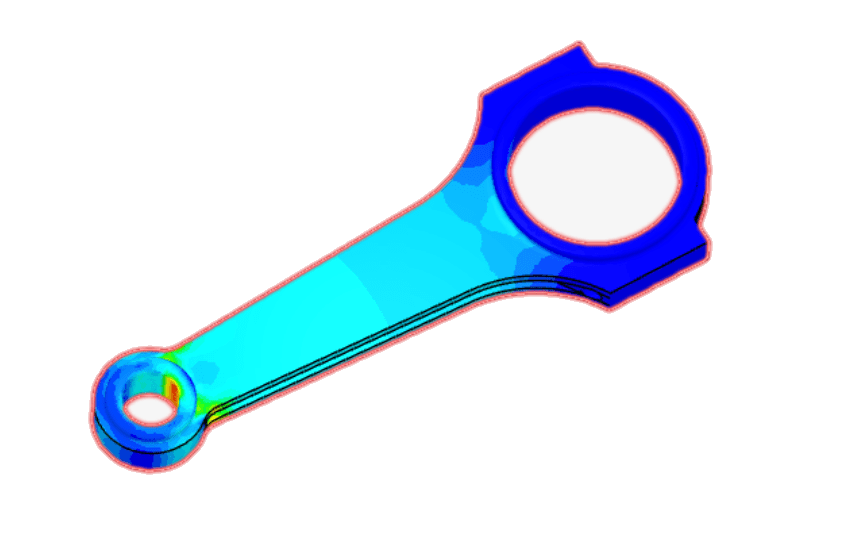
SimScale’s integrated post-processor consists of filters and different viewing tools to better visualize and download the simulation results. Figure 17 shows the default view where the displacement filter is applied with contours of Von Mises Stress for visualization.
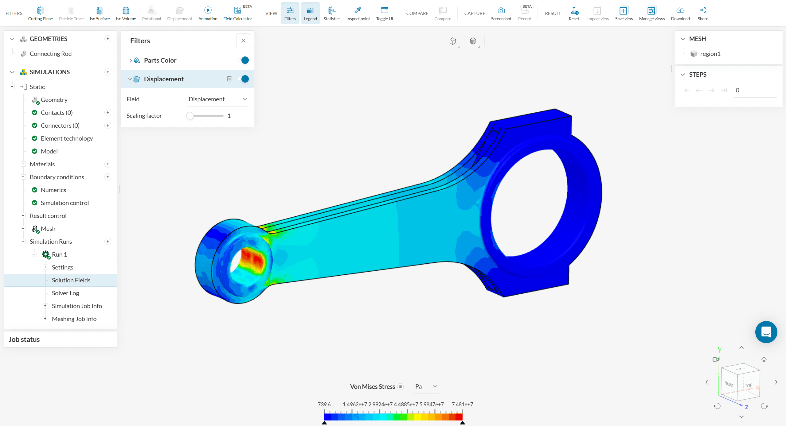
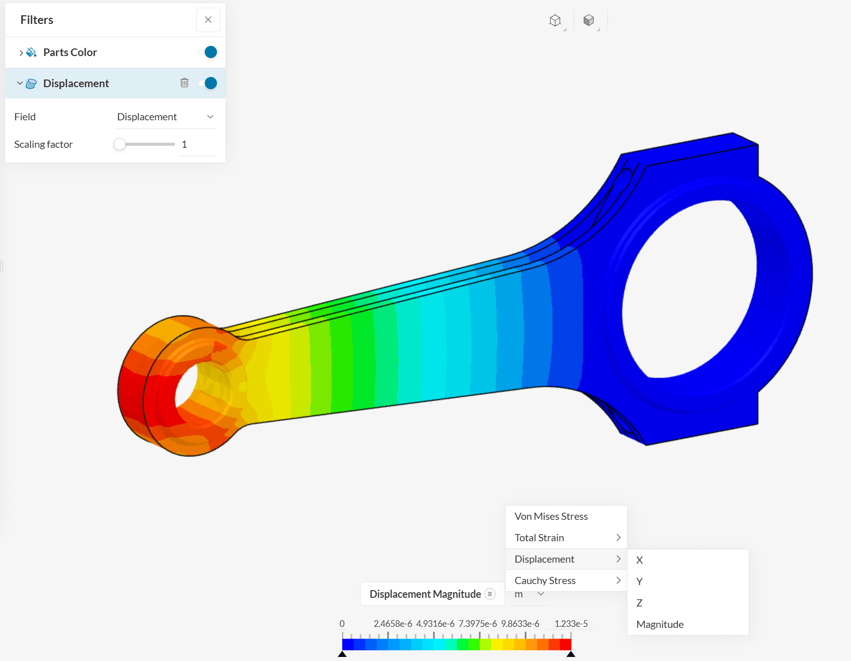
Regions of high stress load are colored red while lower stress regions are shown in blue. The legend can be changed to some other quantity of interest as shown below:
Another common way of displaying linear static FEA results is by creating an animation of the scaled displacement field. Since linear static studies don’t show large displacement levels, a displacement scaling filter can be applied as illustrated by Figure 19.
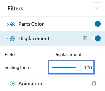
With larger displacements being presented, the animation filter will produce a useful visualization of the part’s deformation behavior. To enable the animation filter for the geometry’s scaled and deformed shape, click ‘Animation’ > ‘Animation Type’ > ‘Shape’.
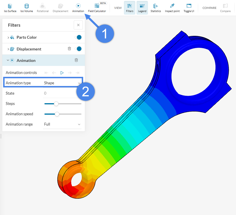
The obtained result is illustrated by Animation 1.
Congratulations! You just finished a Stress Analysis simulation on SimScale!
Find more tutorials, including a more detailed post-processing tutorial with the connecting rod geometry, on our website: SimScale Tutorials and User Guide
Last updated: February 12th, 2026
We appreciate and value your feedback.
Sign up for SimScale
and start simulating now