K-Epsilon Turbulence Models
SimScale allows different methods to model the turbulent effects appearing in a CFD simulation. The SimScale CFD solver uses its in-house version of the widely accepted industry standard turbulence models. This document sheds light on the popular k-epsilon turbulence models.
Overview
The Reynolds-averaged Navier Stokes (RANS) equation in tensor form\(^1\) can be written as:
$$ {\frac{\partial (\rho U_i)}{\partial t}} + {\frac{\partial (\rho U_iU_j)}{\partial x_j}} = -\frac{\partial P}{\partial x_i} + {\frac{\partial}{\partial x _ j}\left[\mu\left(\frac{\partial U _ i}{\partial x _ j} + \frac{\partial U _ j}{\partial x _ i}\right) – \rho \overline{{u_i}'{u_j}’}\right]} \tag{1} $$
where,
- \(U\) = mean flow velocity
- \(u’\) = velocity fluctuations due to turbulence
- \(\mu\) = molecular viscosity
- \(-\rho \overline{{u_i}'{u_j}’}\) = Reynolds Stress term
The Reynolds averaging process results in an additional stress term – Reynolds Stress. To solve the RANS equations we need to express the Reynolds stress in terms of mean flow quantities.
The solution for the Reynolds stress term is given by the Eddy viscosity hypothesis/ Boussinesq hypothesis\(^1\) as
$$-\rho \overline{{u_i}'{u_j}’} = \mu_t\left(\frac{\partial U_i}{\partial x_j}+ \frac{\partial U_j}{\partial x_i} -\frac{2}{3}\frac{\partial U_k}{\partial x_k} \delta_{ij} \right) -\frac{2}{3} \rho k \delta_{ij} \tag{2}$$
where,
- \(\mu_t\) = turbulent or eddy viscosity
- \(\delta_{ij}\) = Kronecker Delta
$$ \delta_{ij} =
\begin{cases}
1, & \text{if $i=j$ \(\to\) Normal stress component} \\[2ex]
0, & \text{if $i \neq j$ \(\to\) Shear stress component}
\end{cases}$$
Equation 2 is a combined equation for the shear and normal components of Reynolds stresses. Observing equation 2 we realize that once we solve for the turbulent viscosity \((\mu_t)\) we can solve the RANS equation 1.
Hence, the difference between different turbulent models is the methodology to calculate turbulent viscosity.
K-Epsilon Turbulence Models
The k-epsilon (\(k-\epsilon\)) model for turbulence is the most common to simulate the mean flow characteristics for turbulent flow conditions. It is an Eddy viscosity model which is a class of turbulence models used to calculate the Reynolds stresses.
It is a two-equation model. That means in addition to the conservation equations, it solves two transport equations (PDEs), which account for the historical effects like convection and diffusion of turbulent energy. The two transported variables are turbulent kinetic energy (\(k\)), which determines the energy in turbulence, and turbulent dissipation rate (\(\epsilon\)), which determines the rate of dissipation of turbulent kinetic energy.
Different variations of the k-epsilon model exist such as Standard, Realizable, RNG, etc. each with certain modifications to perform better under certain fluid flow conditions. In SimScale, the standard and realizable versions are available.
Standard K-Epsilon Model
Transport Equations for the Turbulence Variables
The transport equation for turbulent kinetic energy is given by\(^2\)
$$ {\frac{\partial (\rho k)}{\partial t}} + {\frac{\partial (\rho U_ik)}{\partial x_i}} = {\frac{\partial}{\partial x _j}}\left[\left(\mu+\frac{\mu_t}{\sigma_k} \right){\frac{\partial k}{\partial x_j}}\right] + P_k + P_b -\rho \epsilon +S_k \tag{3} $$
where,
- \(P_k\) = production of turbulent kinetic energy (TKE) due to mean velocity shear
- \(P_b\) = production of TKE due to buoyancy
- \(S_k\) = user-defined source
- \(\sigma_k\) = turbulent Prandtl number for \(k\)
The transport equation for the turbulent dissipation rate is given by\(^2\)
$$ {\frac{\partial (\rho \epsilon)}{\partial t}} + {\frac{\partial (\rho U_i \epsilon)}{\partial x_i}} = {\frac{\partial}{\partial x _j}}\left[\left(\mu+\frac{\mu_t}{\sigma_\epsilon} \right){\frac{\partial \epsilon}{\partial x_j}}\right] + C_1 \frac{\epsilon}{k}(P_k +C_3P_b) -C_2 \rho \frac{\epsilon^2}{k} + S_\epsilon \tag{4} $$
where,
- \(C_1, C_2, C_3, C_\mu\) are model coefficients that vary within \(k-\epsilon\) turbulence models
- \(S_\epsilon\) = user-defined source
- \(\sigma_\epsilon\) = turbulent Prandtl number for \(\epsilon\)
Modeling Turbulent Viscosity
Older turbulence models used a mixing length approach to solve for the turbulent (Eddy) viscosity. The \(k-\epsilon\) turbulence model solves for the turbulence dissipation rate instead.
The turbulent energy \(k\) is given by:
$$k=\frac { 3 }{ 2 } { \left( UI \right) }^{ 2 }\tag{5}$$
where \(U\) is the mean flow velocity and \(I\) is the turbulence intensity.
The turbulence intensity gives the level of turbulence and can be defined as follows:
$$I = \frac { u’ }{ U }\tag{6}$$
where \(u’\) is the root-mean-square of the turbulent velocity fluctuations given as:
$$u’ = \sqrt { \frac { 1 }{ 3 } \left( { { u’ }_{ x } }^{ 2 } + { { u’ }_{ y } }^{ 2 } + { { u’ }_{ z } }^{ 2 } \right) } =\sqrt { \frac { 2 }{ 3 } k }\tag{7}$$
The mean velocity \(U\) can be calculated as follows:
$$U = \sqrt { { { U }_{ x } }^{ 2 }+{ { U }_{ y } }^{ 2 }+{ { U }_{ z } }^{ 2 }}\tag{8}$$
The specific turbulent dissipation rate can be calculated using the following formula:
$$\epsilon ={ { C }_{ \mu } }^{ \frac { 3 }{ 4 } }\frac { { k }^{ \frac { 3 }{ 2 } } }{ l }\tag{9}$$
where \({ { C }_{ \mu } }\) is the turbulence model constant, \(l\) is the turbulent length scale.
The turbulence length scale describes the size of large energy-containing eddies in a turbulent flow.
The turbulent viscosity \(\mu_t\) is, thus, calculated as:
$$\mu_{t} = C_\mu \rho \frac{k^2}{\epsilon}\tag{10}$$
The model coefficients have been derived from experiments and evolved over time. The current-most and widely accepted values are from Launder and Sharma (1974) as follows:
| \(\sigma_k\) | \(\sigma_\epsilon\) | \(C_1\) | \(C_2\) | \(C_\mu\) |
| 1 | 1.3 | 1.44 | 1.92 | 0.09 |
Low-Re Formulation
In \(k-\epsilon\) models the model coefficients \(C_1, C_2, C_\mu\) are damped. The damping functions are termed \(f_1, f_2, f_\mu\) respectively and vary between the different solvers. Hence, this turbulence model can also be applied in the viscous sublayer (y+<5). This is called low-Re (low Reynolds number) formulation.\(^2\)
Please note that there are other models like realizable \(k-\epsilon\) or \(k-\omega\ SST\) that perform better and are more capable for flows close to the wall (y+ <5 or <1).
Applications
The \(k-\epsilon\) model is shown to be reliable for free-shear flows, such as the ones with relatively small pressure gradients. It is preferred for high-Re (high Reynolds number) applications (y+ > 30) where separations and reattachments of the flows are not present.
The standard model might not be the best model for problems involving adverse pressure gradients, large separations, reattachments, axisymmetric jets and complex flows with strong curvatures.
Realizable K-Epsilon Model
The Standard \(k-\epsilon\) model is not preferred for flows close to the wall (y+ <5 or <1) as it is found to not accurately capture the wall shear stresses.
The Realizable \(k-\epsilon\) turbulence model was developed to overcome the shortcomings of the standard model by satisfying mathematical constraints on the Reynolds stresses, consistent with the physics of turbulent flows.
Transport Equations for the Turbulence Variables
The transport equation for the turbulent kinetic energy remains same between the standard and realizable \(k-\epsilon\) models (see equation 3 ). The transport equation for the dissipation rate, however, changes for the realizable model and is given by\(^3\):
$$ {\frac{\partial (\rho \epsilon)}{\partial t}} + {\frac{\partial (\rho U_i \epsilon)}{\partial x_i}} = {\frac{\partial}{\partial x _j}}\left[\left(\mu+\frac{\mu_t}{\sigma_\epsilon} \right){\frac{\partial \epsilon}{\partial x_j}}\right] + \rho C_1S_\epsilon -C_2 \rho \frac{\epsilon^2}{k+\sqrt{\nu\epsilon}} + C_1 \frac{\epsilon}{k}C_3P_b + S_\epsilon \tag{11} $$
Comparing the dissipation rate equations for standard and realizable \(k-\epsilon\)
The major differences in equation 11 compared to equation 4 are the absence of the production term \(P_k\) and the absence of singularity in the denominator \((k+\sqrt{\nu\epsilon})\) of the destruction term i.e. the denominator never vanishes even if \(k\) vanishes. These differences are said to benefit the realizable \(k-\epsilon\) model in accurately predicting energy transfer.
Modeling Turbulent Viscosity
The turbulent viscosity \((\mu_t)\) is calculated similarly to equation 10, however, \(C_\mu\) is no longer a constant as in the standard \(k-\epsilon\) model. It is a function of the mean strain and rotation rates from the angular velocity of the system rotation, and the turbulence fields \(k\) and \(\epsilon\).
The values for \(C_1, C_2, \sigma_k, \sigma_\epsilon\) remain the same as discussed in Table 1.
Applications
The Realizable \(k-\epsilon\) model has been validated to outperform the standard model in rotating homogeneous shear flows, free flows including jets and mixing layers, channel and boundary layer flows, and separation and recirculation.
One drawback of the realizable model is that it gives non-physical values for turbulent viscosities in simulations involving stationary and rotatory zones (MRF and AMI rotating zones). This is because \(C_\mu\) in the calculation for \(\mu_t\) includes the effects of mean rotation giving an extra rotation effect.
Inlet Turbulence
To realistically model a given problem, it is important to define the turbulence intensity at the inlets. Here are a few examples of common estimations of the incoming turbulence intensity:
- High-turbulence (between 5% and 20%): Cases with high-velocity flow inside complex geometries. Examples: heat exchangers, flow in rotating machinery like fans, engines, etc.
- Medium-turbulence (between 1% and 5%): Flow in not-so-complex geometries or low speed flows. Examples: flow in large pipes, ventilation flows, etc.
- Low-turbulence (well below 1%): Cases with fluids that stand still or highly viscous fluids, very high-quality wind tunnels. Examples: external flow across cars, submarines, aircraft, etc.
Did you know?
The turbulent intensity at the core of a pipe for a fully developed pipe flow can be estimated as follows:
$$I=0.16 { { Re }_{ { d }_{ h } } }^{ -\frac { 1 }{ 8 } }\tag{12}$$
where \({ { Re }_{ { d }_{ h } } }\) is the Reynolds number for a pipe of hydraulic diameter \({ { d }_{ h } }\).
The turbulence length scale in this case is
$$l=0.07{ d }_{ h }\tag{13}$$
Applying K-Epsilon Model in SimScale
The k-epsilon turbulence model needs to be chosen at the beginning of the simulation setup, in the global settings panel. This is shown in the figure below:
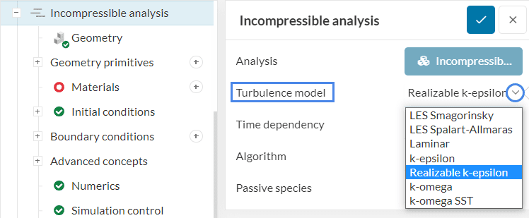
The standard k-epsilon turbulence model is available to all the CFD analysis types and the realizable k-epsilon model is available to the incompressible analysis type.
By default, SimScale defines the initial values of turbulence variables \(k\) and \(\epsilon\) depending on the domain of the problem. If needed, they can be changed under Initial conditions. Further, if the user wants to specifically define the boundary conditions for these turbulence variables, then the custom boundary condition can be used.
References
- “[CFD] Eddy Viscosity Models for RANS and LES.” Fluid Mechanics 101. February 24, 2021.
- “[CFD] The k – epsilon Turbulence Model.” Fluid Mechanics 101. June 15, 2019.
- 12.4.1 Standard k-epsilon model overview – UW courses web server
- B. E. Launder and B. I. Sharma, “Application of the energy dissipation model of turbulence to the calculation of flow near a spinning disc”, Letters in Heat and Mass Transfer, 1974, 1, pp. 131-138, 1974.
- Bardina, J.E., Huang, P.G., Coakley, T.J., “Turbulence Modeling Validation, Testing, and Development”, NASA Technical Memorandum 110446, 1997.
- Wilcox, David C, “Turbulence Modeling for CFD”. Second edition. Anaheim: DCW Industries, pp. 174, 1998.
- https://www.cfd-online.com/Wiki/Turbulence_free-stream_boundary_conditions
Last updated: July 20th, 2023
Did this article solve your issue?
How can we do better?
We appreciate and value your feedback.


