Validation Case: RF Electronics Package Cooling

This study aims at validating the CHT v2 and CHT (IBM) solvers. A peer-reviewed publication of R.Boukhanouf\(^1\) focusing on thermal analyses and cooling of a Radio Frequency (RF) electronics package has been used as the basis for this validation case. Reasonable assumptions and approximations have been made to bridge uncertainty in the publication.

The validation study involves qualitative and quantitative comparisons between SimScale and the commercial CFD code FloTHERM involving:

• temperature, and
• velocity vectors

Geometry

The battery pack was modeled using the CAD tool Onshape. Necessary assumptions were made to overcome missing/inconsistent geometric data:

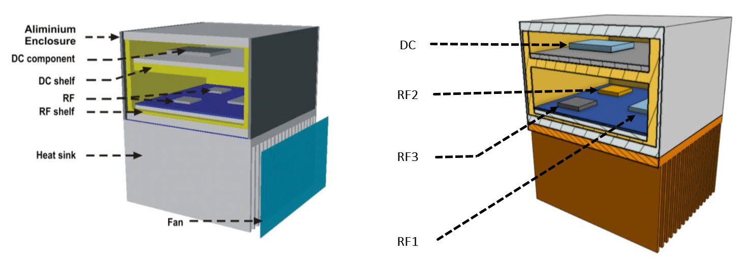
The model contains the following parts:

• DC Shelf
  • Upper Copper mount for DC component
• DC Shelf components
  • DC component with 15 \(W\) Heat Rating
  • Thermal via circuit built into RF4 PCB
  • Solder layer
  • Thermal insulating material (TIM)
• RF Shelf
  • Upper Copper mount for RF components
• RF components
  • Three RF components with 60 \(W\) , 0.5 \(W\), 0.5 \(W\) Heat Ratings
  • Aluminium RF4 PCB
  • Dielectric substrate to insulate components from each other
  • Solder layer
  • Thermal insulating material (TIM)
• Heat sink: Finned Heat Exchanger  
• Aluminium Enclosure Box
• Fan: Air delivery 11 \(m^3 \over \ h\) at 40 \(^o C\)

Analysis Type and Mesh

Tool Type: OpenFOAMⓇ

Analysis Type: Incompressible, steady-state analysis with the Conjugate Heat Transfer v2 (CHT v2) and Conjugate Heat Transfer (IBM) solvers.

Mesh and Element Types:

The Standard mesher algorithm with tetrahedral and hexahedral cells was used to generate the mesh for the CHTv2 runs. Meanwhile, CHT (IBM) uses cartesian meshes:

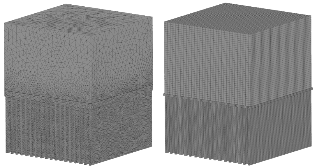
A mesh sensitivity analysis has been carried out to determine the dependence of the CHTv2 solver temperature predictions on the mesh:

	Mesh Count	Mesh Type	TC@DC Component \([°C]\)	TC@RF1 Component \([°C]\)	TC@RF2 Component \([°C]\)	TC@RF3 Component \([°C]\)
Mesh 1	3.4M cells, 1M nodes	Standard	106.72	148.85	88.25	88.25
Mesh 2	4.4M cells, 1.2M nodes	Standard	105.95	148.65	87.75	87.75
Absolute TC deviation (Mesh2-Mesh1)			0.77	0.2	0.5	0.5
% TC deviation (Mesh2-Mesh1)			0.73%	0.13%	0.57%	0.57%

TC stands for the Temperature in Celsius degrees. The values in the table are area-averaged values over the respective components.

It is indicated that the temperature deviation between Mesh 1 and Mesh 2 was found to be within 1% for all the package components:

Simulation Setup

Fluid Material:

• Air
  • Dynamic viscosity \((\mu)\) = 1.83e-5 \(m^2 \over\ s\)
  • Specific heat = 1004 \(J \over\ (kg \times\ K)\)

Solid Materials:
The table highlights the materials and thermal conductivity values used for each component of the RF electronics package:

Component	Material	Thermal conductivity \(W \over \ (m \times \ K) \)
Enclosure Box	Aluminum	180
RF & DC shelves	Copper	385
Solder layer	Tin	50
Thermal via circuit	(Derived)	22 (Derived)
TIM	Sil Pad® and Gap Pad®	2
Dielectric Substrate	Dielectric material	0.6
PCB	Aluminum	180

The RF components have been modeled as using the thermal resistance network and therefore are not assigned any material properties.

The Heat Ratings and Thermal Resistance values used are respectively as follows:

• RF1: 15 \(W\), 0.7 \(^o C \over \ W\) 
• RF2: 0.5 \(W\), 0.8 \(^o C \over \ W\)  
• RF3: 0.5 \(W\), 0.8 \(^o C \over \ W\) 
• DC: 60 \(W\), 0.78 \(^o C \over \ W\)

Boundary Conditions:

• Natural convection inlet-outlet with an ambient temperature of 40 \(^o C\)
• Fan as a momentum source with a velocity of 1.85 \(m \over \ s\)
• Thermal Resistance Network: Star Network Resistance Model
• DC Component:
  • Resistance: 0.78 \(K \over \ W\)
  • Power Source: 15 \(W\)
• RF1 Component:
  • Resistance: 0.7 \(K \over \ W\)
  • Power Source: 60 \(W\)
• RF2 Component:
  • Resistance: 0.8 \(K \over \ W\)
  • Power Source: 0.5 \(W\)
• RF2 Component:
  • Resistance: 0.8 \(K \over \ W\)
  • Power Source: 0.5 \(W\)
• No-slip walls
• Coupled contact interfaces

Result Comparison

Convergence below 1e-3 has been achieved. Calculated physical quantities such as inlet pressure, outlet velocity, and cell average temperatures have also been allowed to converge to stable values.

The validation of the SimScale’s CHTv2 has been carried out by qualitatively comparing temperatures and velocities with the reference results\(^1\). The reference results have been produced with the commercial CFD code Flotherm. All post-processing was done in SimScale’s online post-processor:

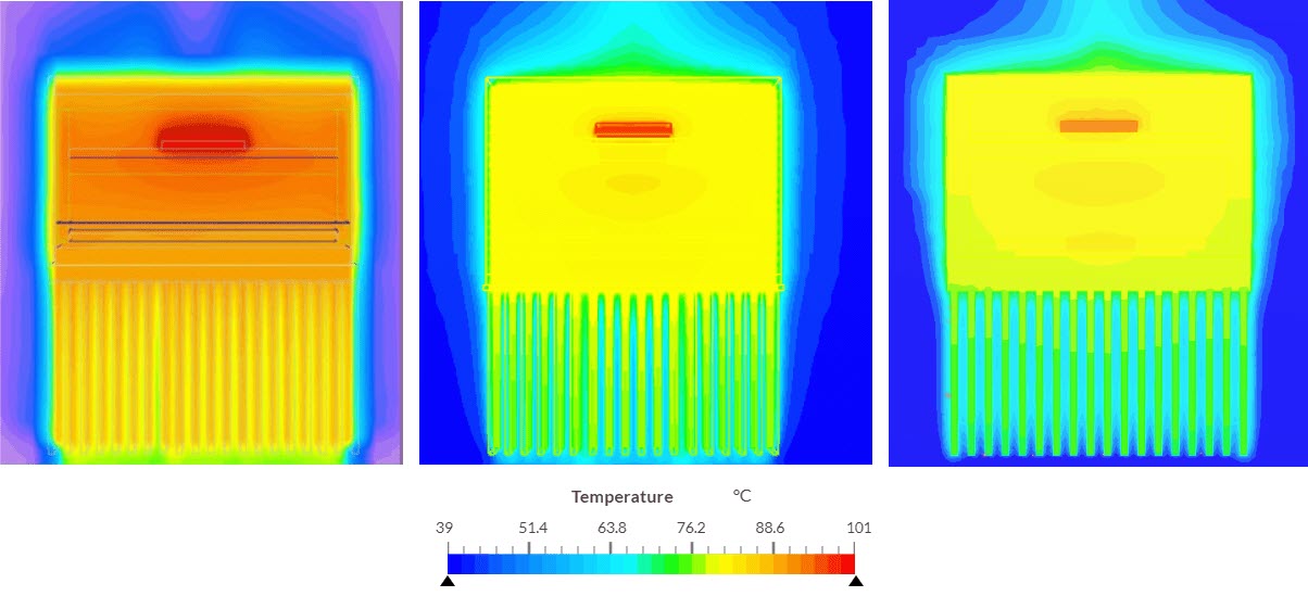
Another section was compared between the two:

A quantitative comparison of the velocity field shows a good match between the two solvers:

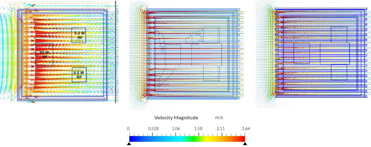
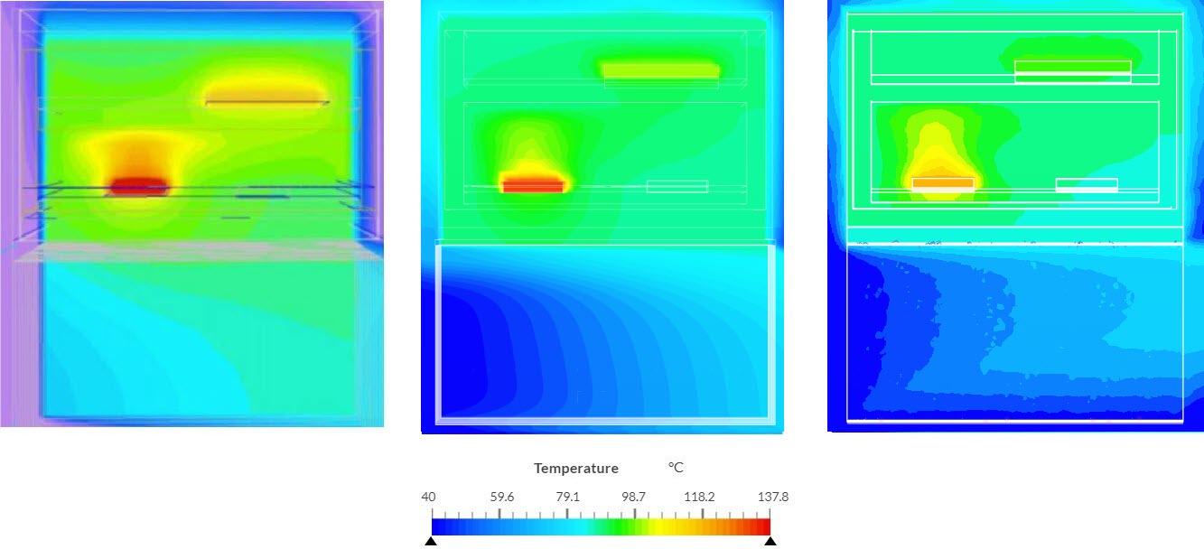
Except from the qualitative comparison, a quantitative study was performed:

Component	FloTHERM \([°C]\)	CHT (IBM) \([°C]\)	CHT v2 \([°C]\)	TC deviation (CHT IBM – FloTHERM) \([°C]\)	TC deviation (CHTv2 – FloTHERM) \([°C]\)
TC@DC Component	101	98.46	105.95	-2.54	4.95
TC@RF1 Component	137.85	133.77	148.65	-4.08	10.8

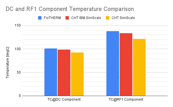
From Table 3 and Figure 7 above, the DC and RF1 component temperatures are within 5% and 8% of the reference FloTHERM results respectively.

This deviation could be traced down to two possible factors:

• The publication does not clarify how the thermal resistance has been implemented (top/board/side). 
• Temperature measurement type in the paper.

Overall, The study shows a moderately good agreement between the temperature predictions from the two CFD solvers.

Last updated: September 8th, 2023