Documentation
This tutorial showcases how to use SimScale to run a Time-Harmonic electromagnetics simulation on a 3-Phase Transformer, where the objective is to ensure efficient AC power transmission and distribution by evaluating the transformer’s performance under sinusoidal steady-state operating conditions.
This tutorial teaches how to:
We are following the typical SimScale workflow:
To begin, click on the button below. It will copy the tutorial project containing the geometry into your Workbench.
The following picture demonstrates what is visible after importing the tutorial project.
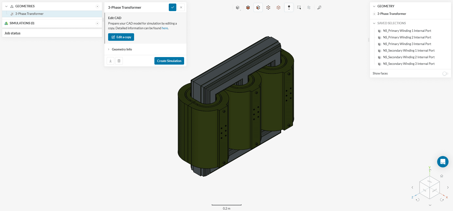
The geometry consists of a linear actuating solenoid. It consists of multiple parts, as can be observed in the scene tree.
The ‘3-Phase Transformer’ geometry requires further preparation for electromagnetic simulation. While the solid components like the coils and core are present, the solver also necessitates a solid representation of the surrounding fluid. This fluid domain will serve as the medium through which the electric and magnetic fields propagate.
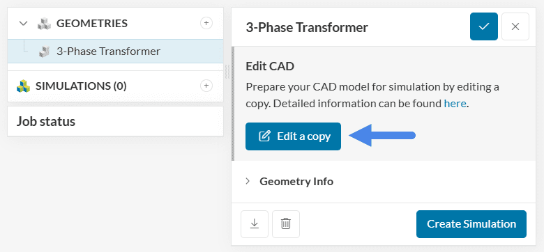
To create a flow volume, click on the ‘Edit a copy’ icon.
Follow the steps below as shown in Figure 4 to create the external flow volume.
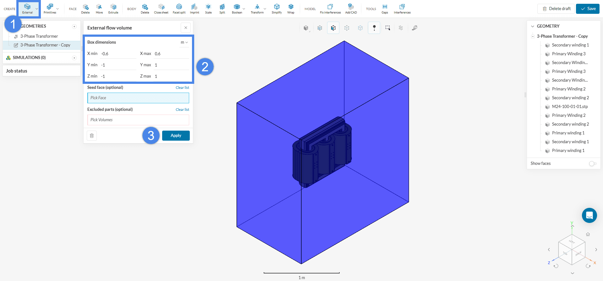
Notice that there is a new volume entity called Flow region under the parts list at the very end (see Figure 5, far right). Use the ‘Save’ button to save this new geometry in the Workbench.
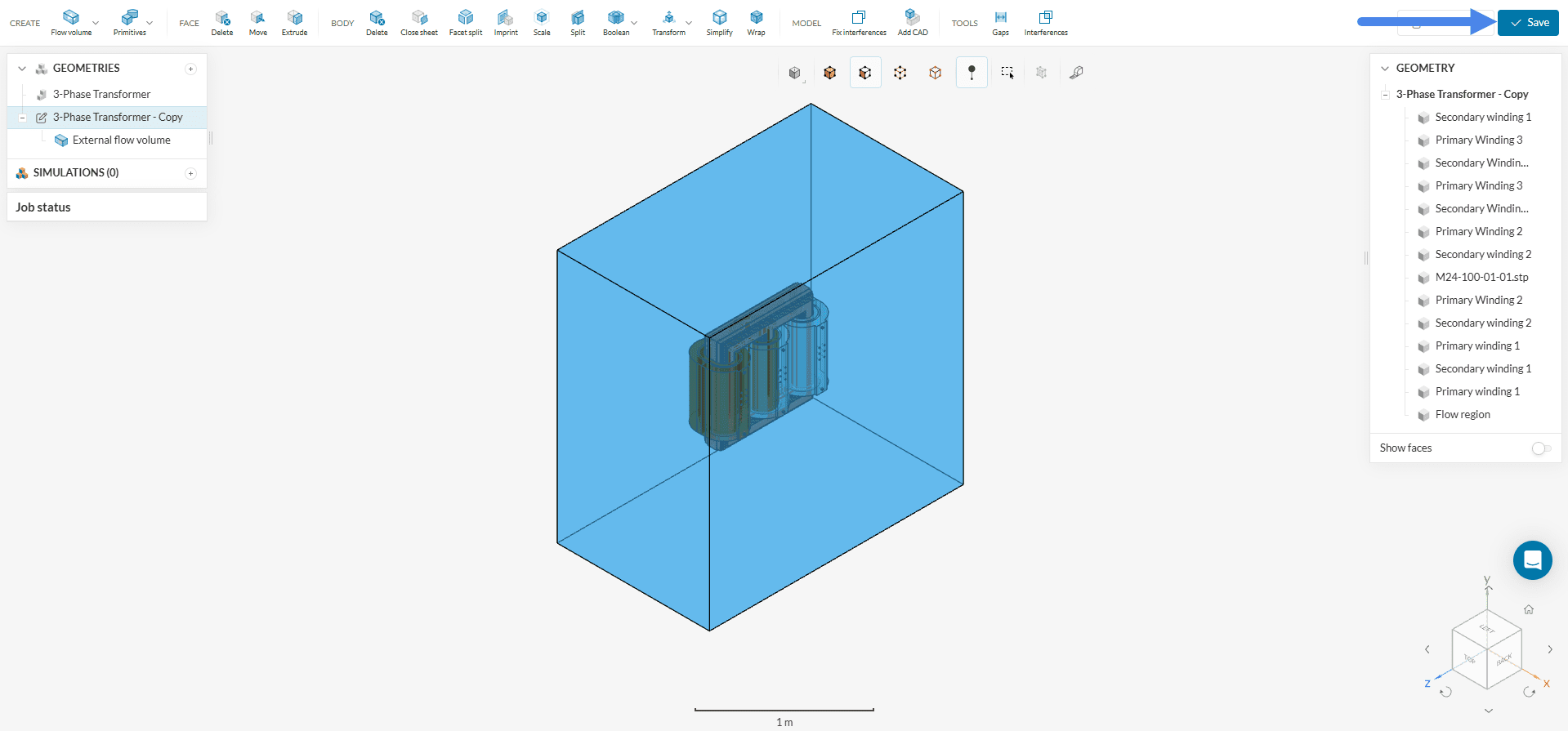
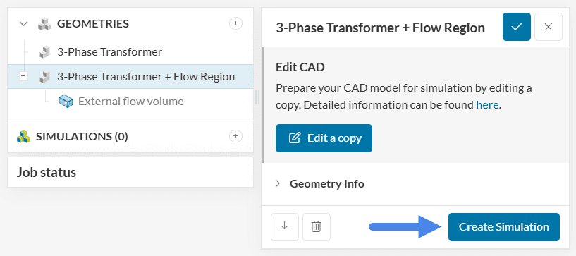
After the save, two geometries are now in the geometry section: 3-Phase Transformer and Copy of 3-Phase Transformer. For better clarity, rename Copy of 3-Phase Transformer as ‘3-Phase Transformer + Flow Region’.
To start the simulation setup process, select the newly saved CAD ‘3-Phase Transformer + Flow Region’ and click on the ‘Create Simulation’ button.
This will open the simulation type selection widget:
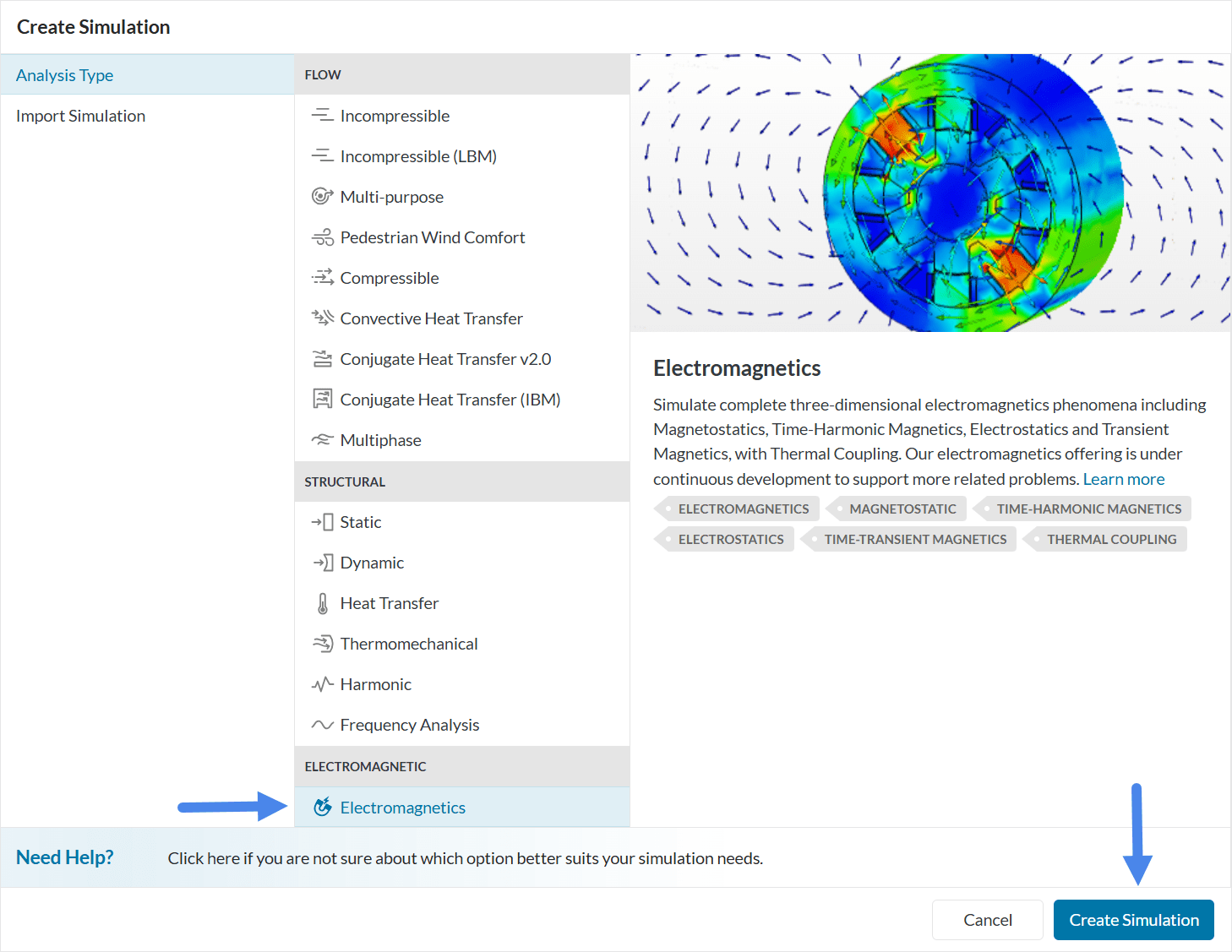
Choose ‘Electromagnetics‘ as the analysis type and ‘Create Simulation’.
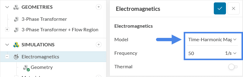
At this point, the simulation tree will be visible on the left-hand side panel.
The initial step in configuring the simulation involves adjusting the global settings of the study. These settings influence how the underlying equations are solved and must be defined at the beginning of each project. In this example, the Model will be set to ‘Time-Harmonic Magnetics’, and the Frequency will be specified as ’50 Hz’.
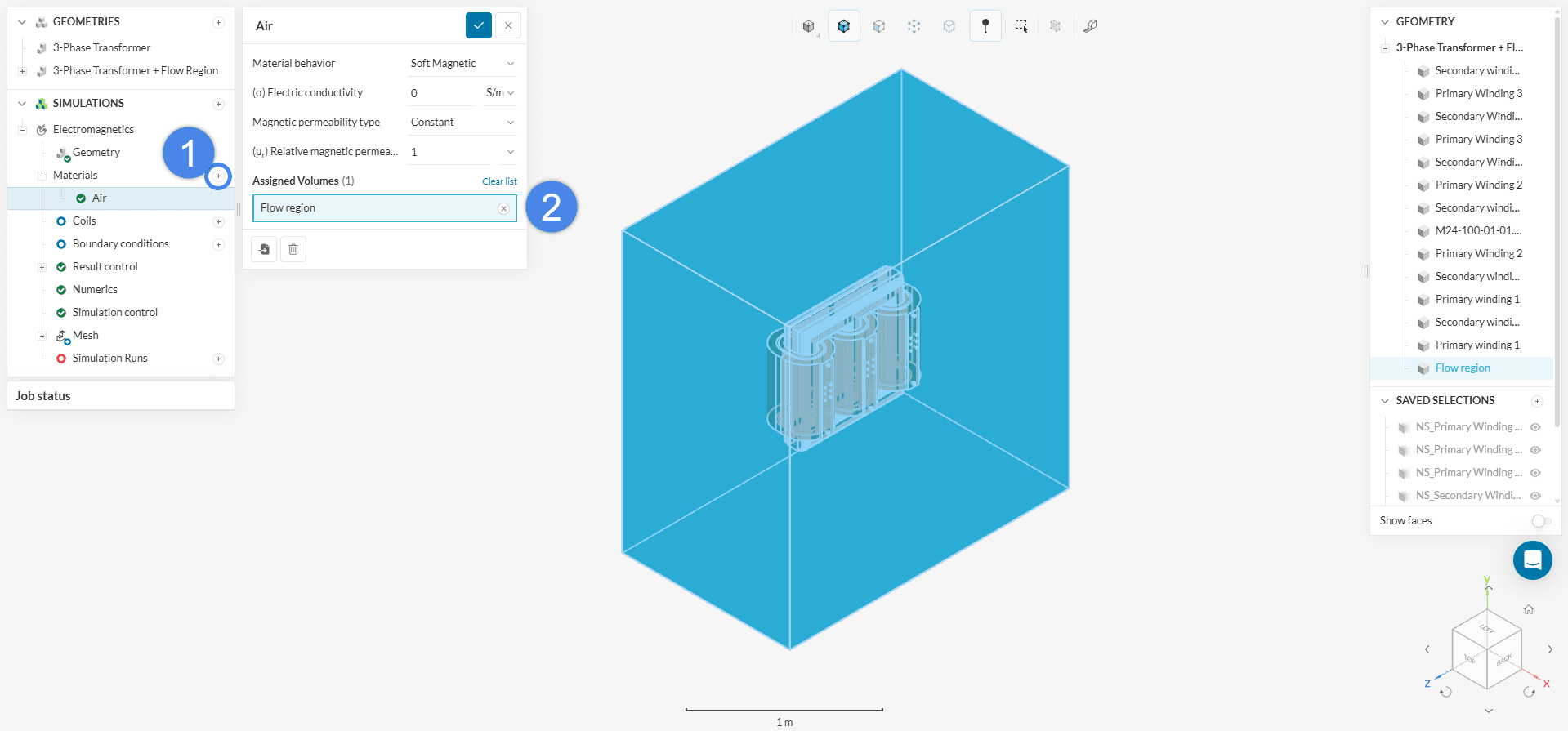
This simulation will begin with air present in the flow region. Then we will assign Copper to the coils and Steel to the core. Therefore, this simulation will use three materials. To start assigning, click on the ‘+’ button next to Materials. In doing so, the SimScale fluid material library opens, as shown in the figure below:
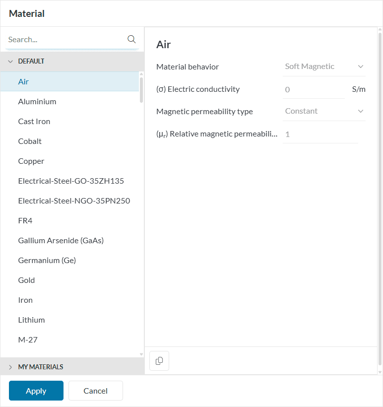
Select ‘Air‘ and click ‘Apply’. This means air will be recognized by the flow region throughout the simulation. Keep the default values, and assign the entire Flow region to it (if not already by default).
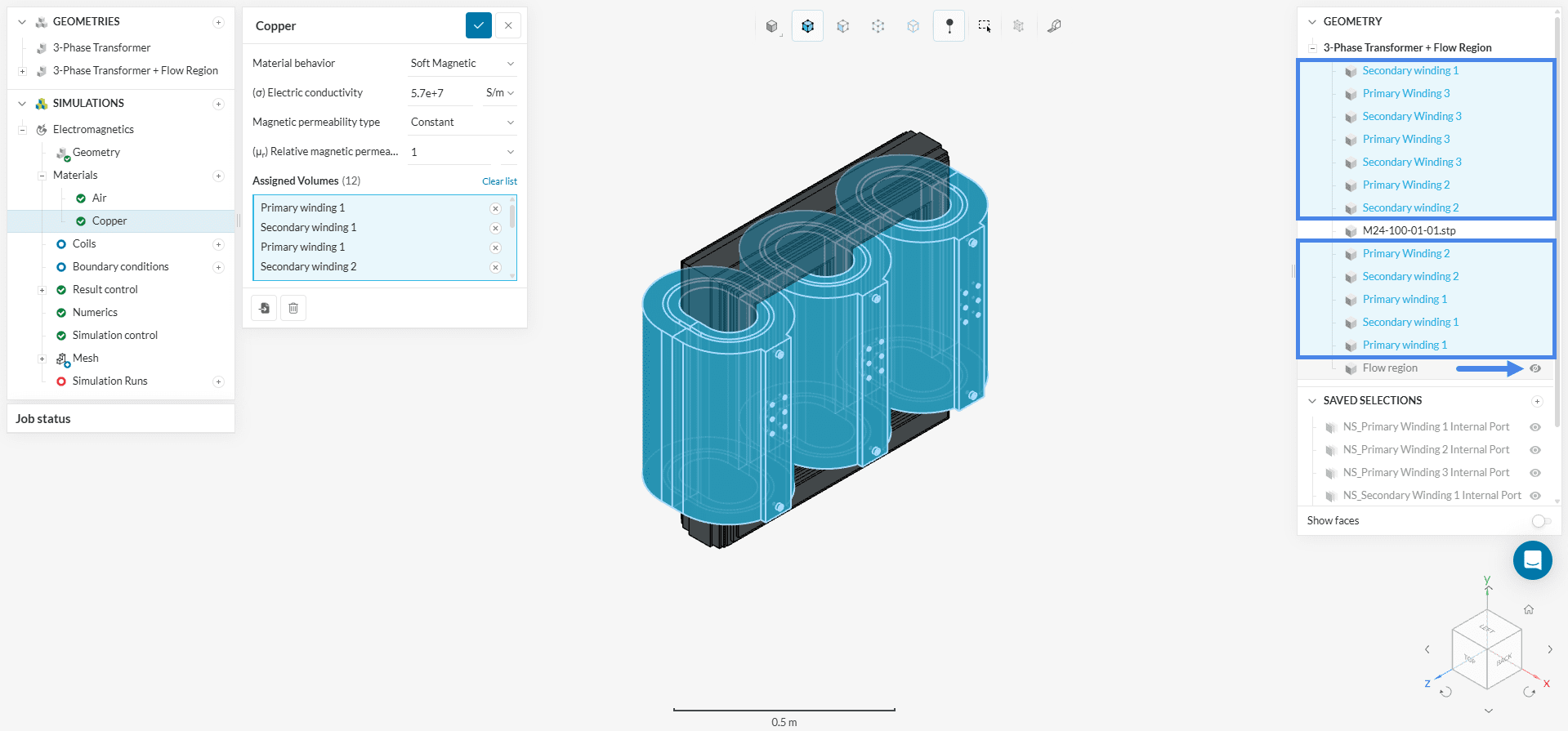
Next, define the material for the coils. To do this, create a new material and select ‘Copper’. Then, as illustrated in the figure below, hide the Flow region and assign the material to the coil volumes.
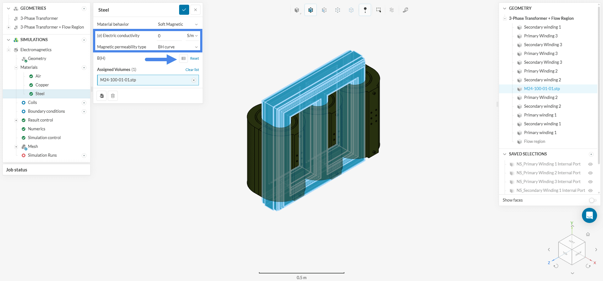
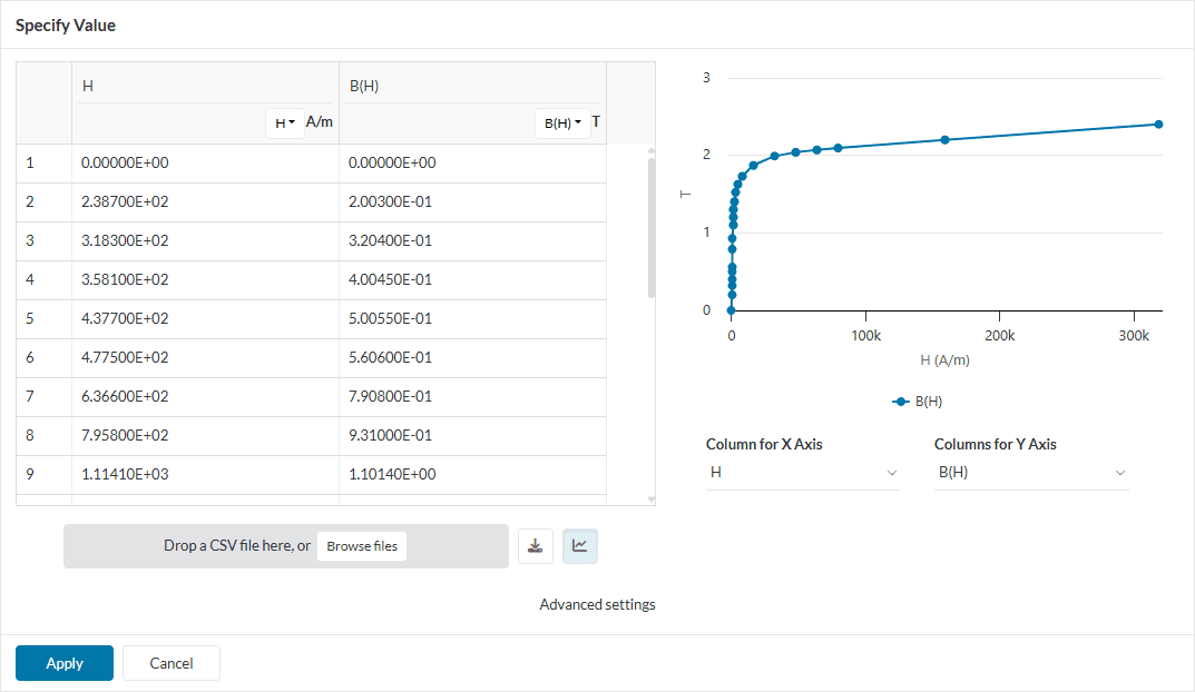
To define the Core material, create a new material and select ‘Steel’. Set the Electric conductivity to ‘0’ \(S/m\) and for the Magnetic permeability type, choose ‘BH curve’. Finally, assign this material to the core and click the table icon to input the BH curve.
You can find the B/H curve for the AISI Steel material below. Figure 13 shows the assigned material table as well as the B/H curve.
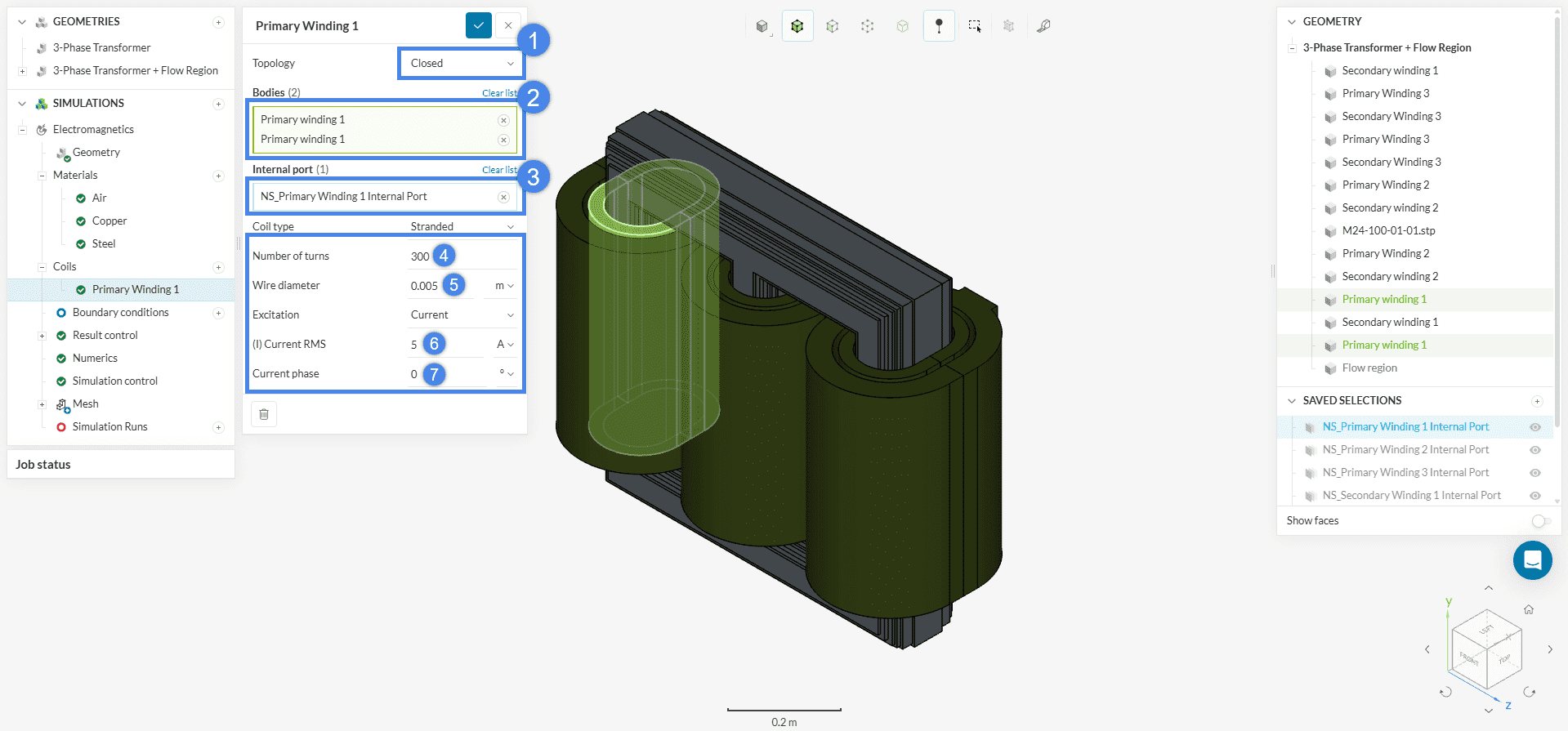
Under Coils in the simulation tree, create a new closed coil. To specify the internal port of the coil it has been cut into two halves, thus both halves are assigned in a single coil setting. Assign the two ‘Primary Winding 1’ solids to Bodies. For the Internal port, an inner face must be selected – you can choose the ‘NS_Primary Winding 1 Internal Port’ saved selection. Then, change the respective values as shown in Figure 14 for Topology, Number of turns, Wire diameters, and (I) Current.
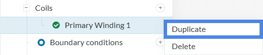
For the remaining primary windings (2 and 3), simply duplicate the existing coil settings by right-clicking on Primary Winding 1 and selecting Duplicate.
The second and third windings have different phase angles compared to the first winding, and this setting must be adjusted under Current phase for those coils (n. 7, Figure 14). Below is a table with the Current Phase values for each coil:
| Winding | Current Phase |
| Primary 1 | 0º |
| Primary 2 | 120º |
| Primary 3 | 240º |
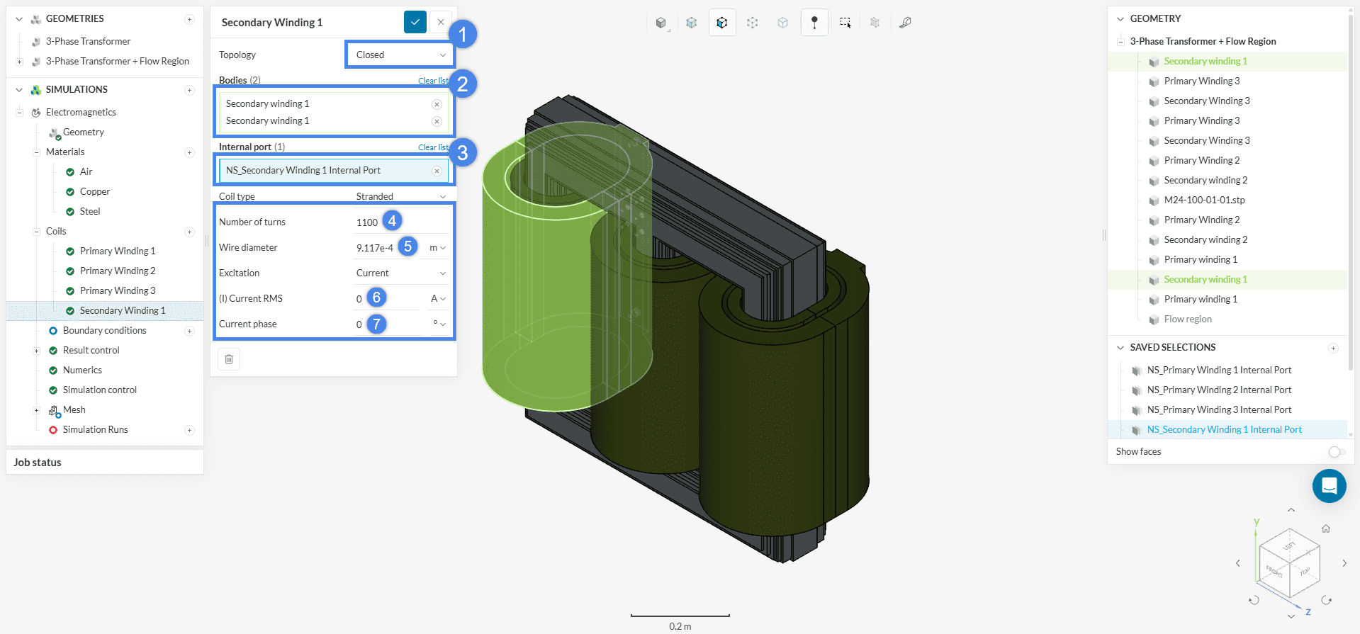
To define the secondary winding coil, simply mimic the steps for setting up the primary winding, adjusting the additional settings as shown in the figure below.
For the second and third secondary windings, input the following values for Current phase:
| Winding | Current Phase |
| Secondary 1 | 0º |
| Secondary 2 | 120º |
| Secondary 3 | 240º |
Tool Tip
By right-clicking on the inside face of the two coils you can use the assign other option to select the hidden inside face of the coil without the need to hide one of the coil parts. More tips and tricks on the selection tools within SimScale can be found here.
There is no need to assign boundary conditions for this simulation.
One of the most important indicators of transformer performance is core saturation. Saturation occurs when a ferromagnetic material (like iron or steel) is exposed to a high magnetic field and reaches a point where most of its magnetic domains are aligned. Beyond this point, further increases in the magnetic field (H) cause only minimal increases in magnetic flux density (B), as seen in the flattening of the B-H curve. At saturation, the material’s permeability drops sharply, reducing its ability to guide magnetic flux efficiently.
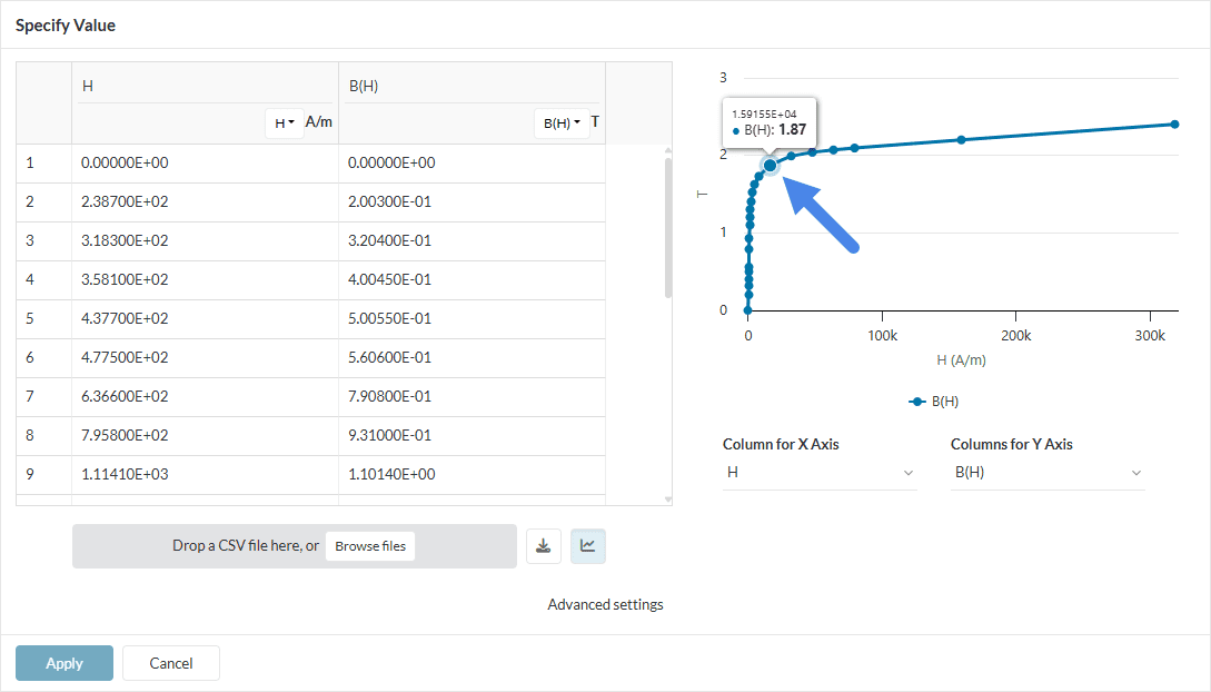
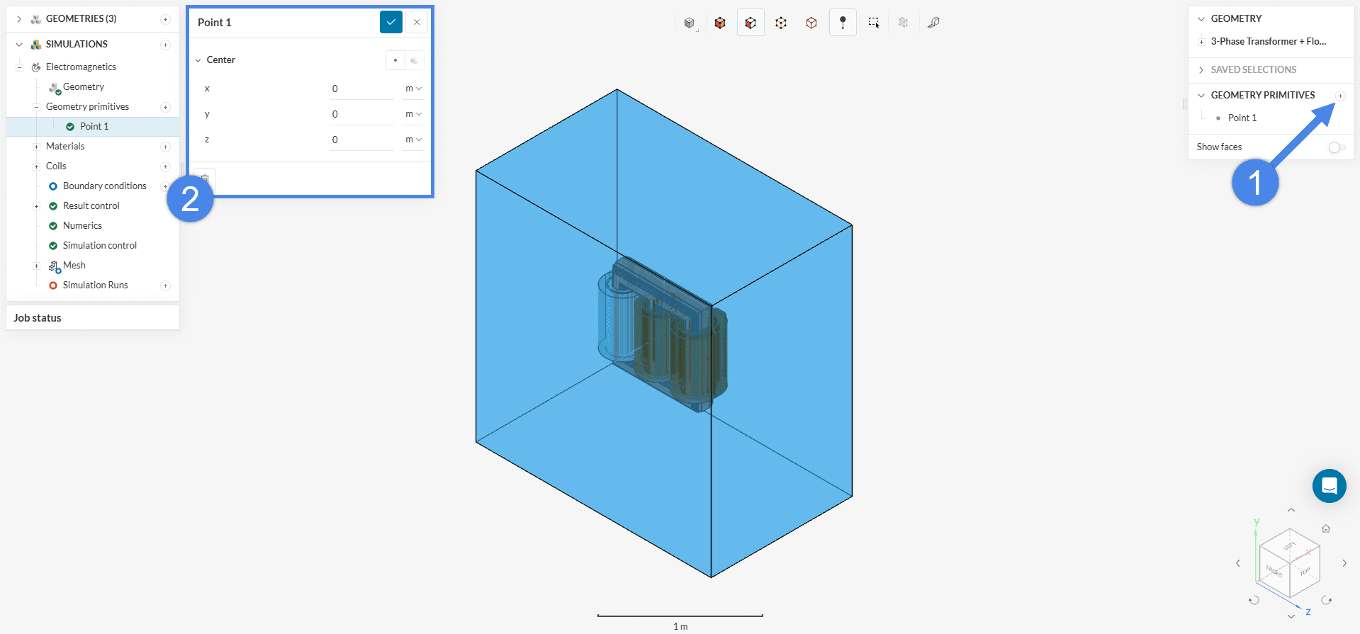
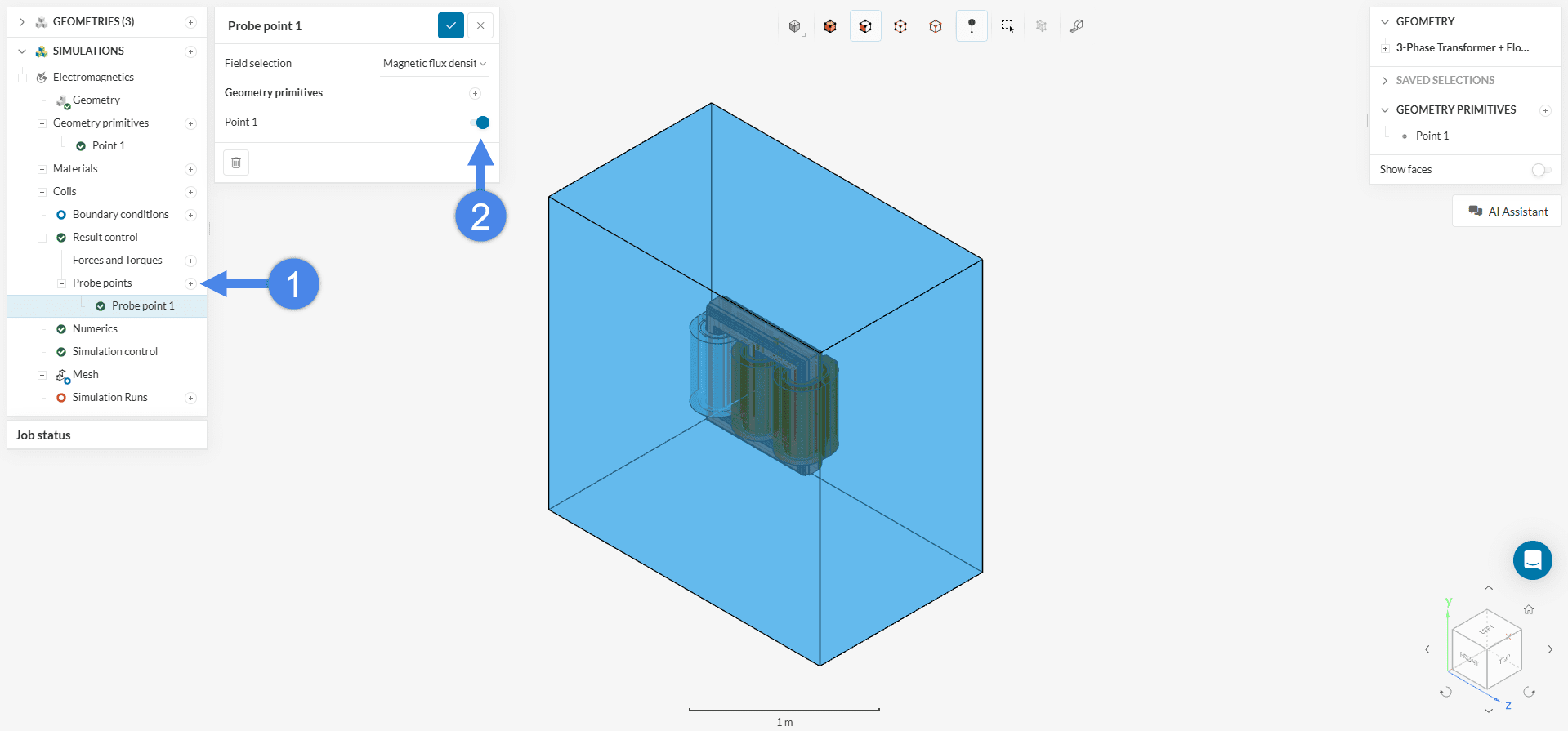
To evaluate this in a 3-phase transformer simulation, we can place a probe point at the center of the core to monitor the magnetic flux density during operation. By comparing the measured value to the material’s saturation threshold from its B-H curve, we can determine whether the core is operating in the linear region or has entered saturation.
To create the point, click the ‘+’ icon next to Geometry Primitives in the Geometry view and select ‘Point’. You can leave the default coordinates (0, 0, 0), as they represent the center of the core.
To create a result control plot using this point, go to Result Control → Probe Points, click ‘+’, and select the point you created earlier. This will enable monitoring of the field variables at that location.
For most analyses, the default settings for Numerics and Simulation control are optimized and do not require modification. The only minor adjustment for this case involves setting the Element accuracy to ‘Second order’ under Numerics. This setting defines a solver interpolation that utilizes second-order (quadratic) shape functions to interpolate electromagnetic field variables (e.g., E, B, etc.) within each element and provides more accurate results at the expense of computational efficiency.
We recommend using the Automatic mesh algorithm for mesh creation. This algorithm is generally a good choice due to its automation and ability to deliver good results for most geometries.
This tutorial will utilize a global mesh fineness level of 3. For users interested in a mesh refinement study, the mesh fineness can be increased by adjusting the Fineness level or by switching the sizing option from Automatic to manual and modifying the edge length range or employing Surface/Volume custom sizing refinements. All these options are described in more detail in the Standard Mesher’s documentation page.
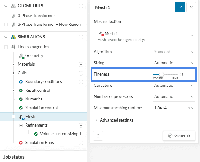
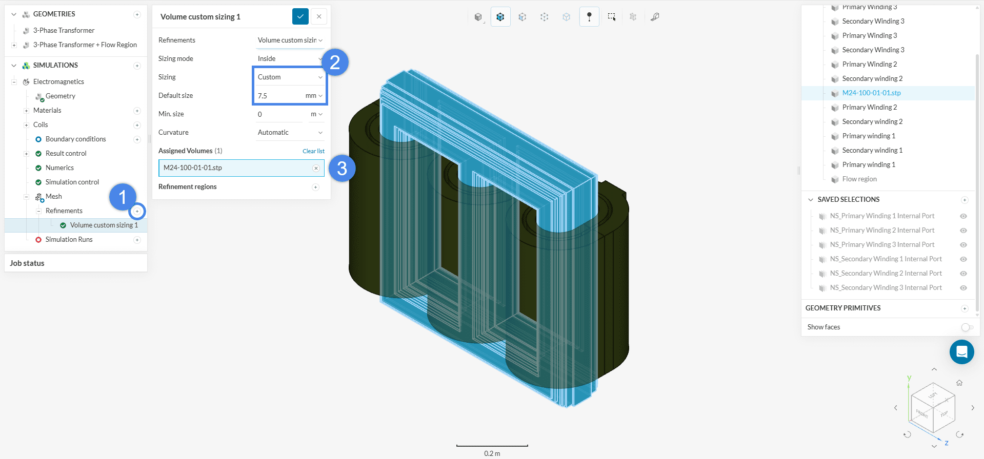
In addition to the mesh fineness of level 3, the core will have a Volume custom sizing refinement with a Default size of ‘7.5’ \(mm\). To do this, create a new refinement and assign the parts as shown in Figure 22.
How can I run a mesh sensitivity study?
As mentioned above, mesh sensitivity studies are essential for validating results and achieving an optimal balance between mesh size and solution accuracy. This article will walk you through the process of setting up such a study.
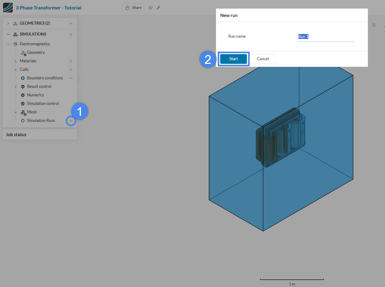
Now you can start the simulation. Click on the ‘+’ icon next to Simulation Runs. This opens up a dialogue box where you can name your run and ‘Start’ the simulation.
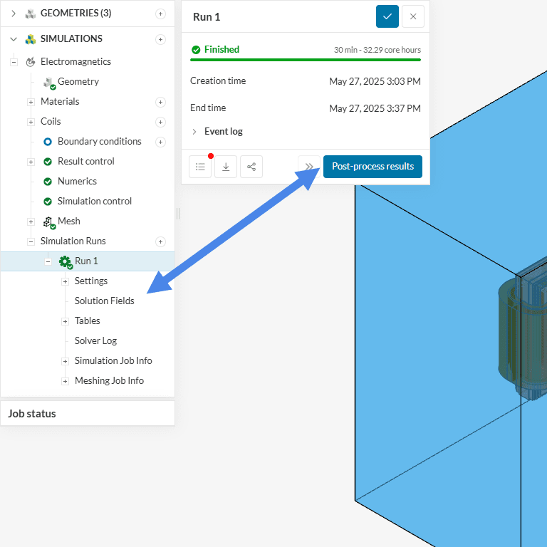
Once the results are calculated and the simulation is over, you can already have a look at them in the post-processor by clicking on ‘Solution Fields’ or ‘Post-process results’, as indicated in Figure 24.
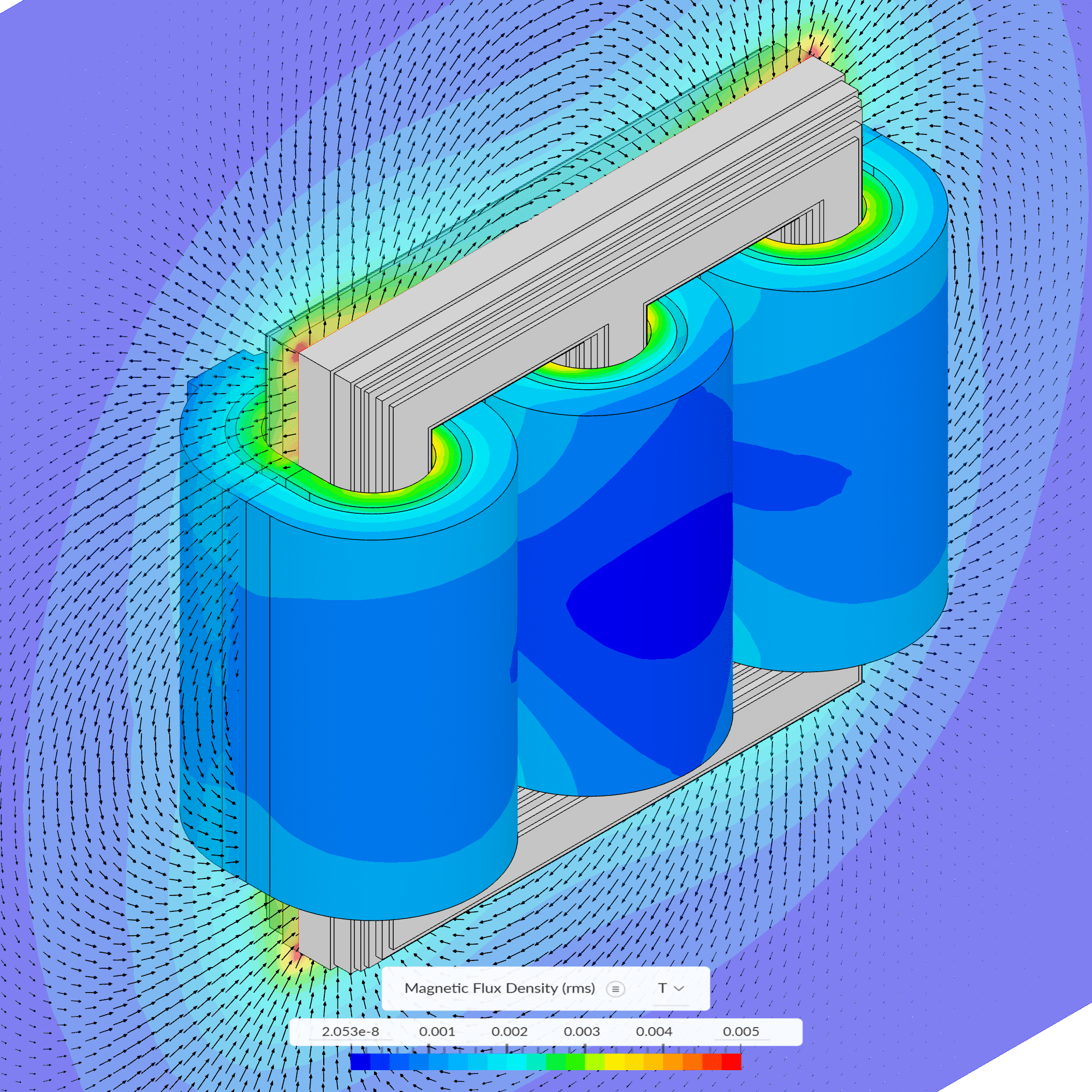
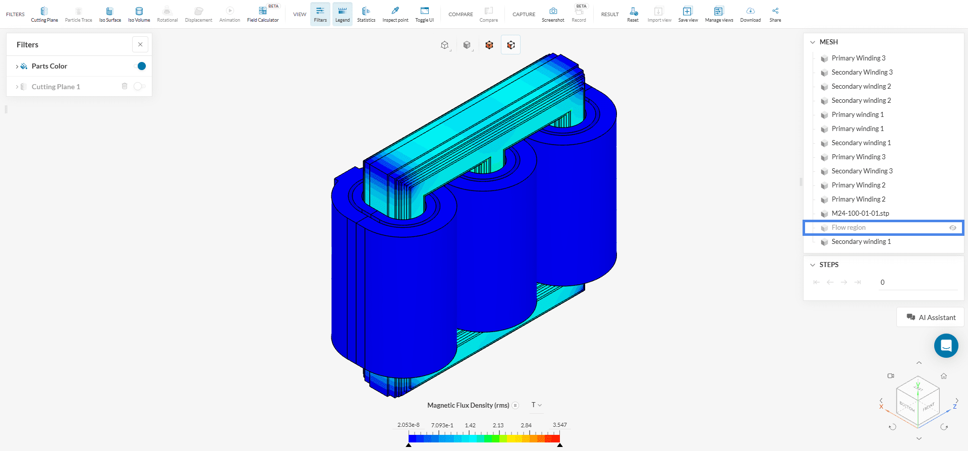
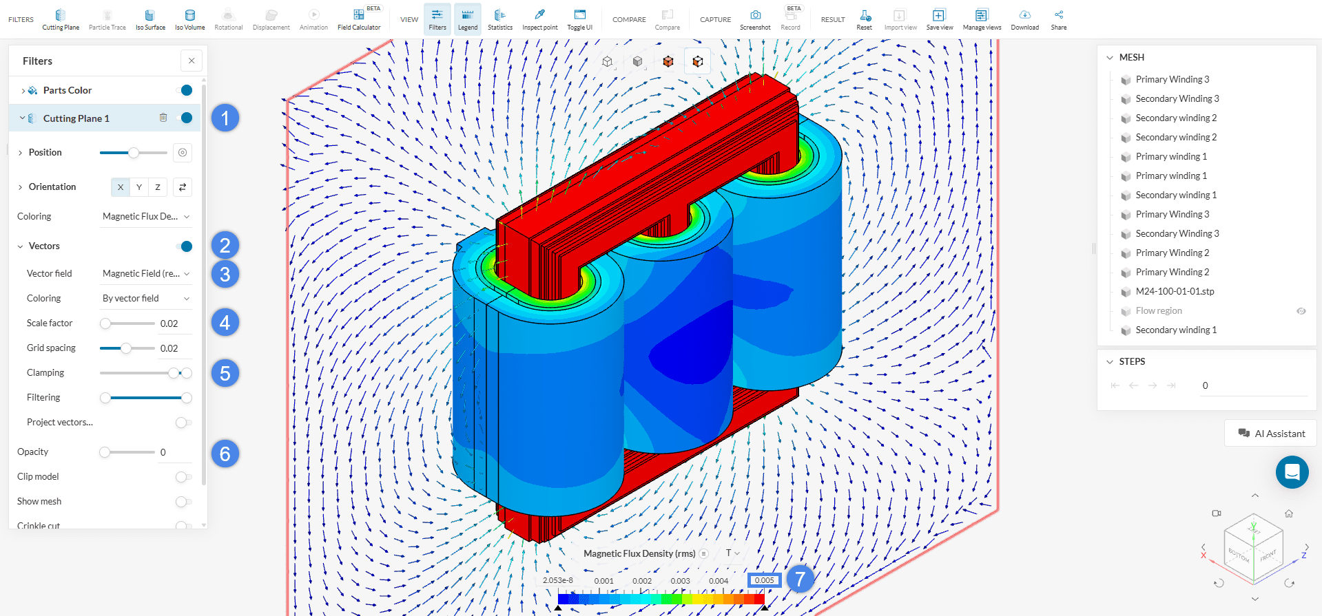
In the post-processor, start by examining the RMS Magnetic Flux Density around the transformer. To do this, turn off the cutting plane, hide the Flow Region, and set Magnetic Flux Density (RMS) as the field shown in the legend.
To visualize the magnetic field around the transformer, re-enable the cutting plane and set its Orientation to the ‘X-direction’. Enable ‘Vectors’, set the vector field to ‘Magnetic Field’, and adjust the Scale factor to ‘0.02’. For better clarity, move the clamping slider to ‘90%’ and set the cutting plane Opacity to ‘0’ so only the vectors remain visible. You can also improve gradient visualization by setting the legend’s upper limit to ‘0.005’ \(T\).
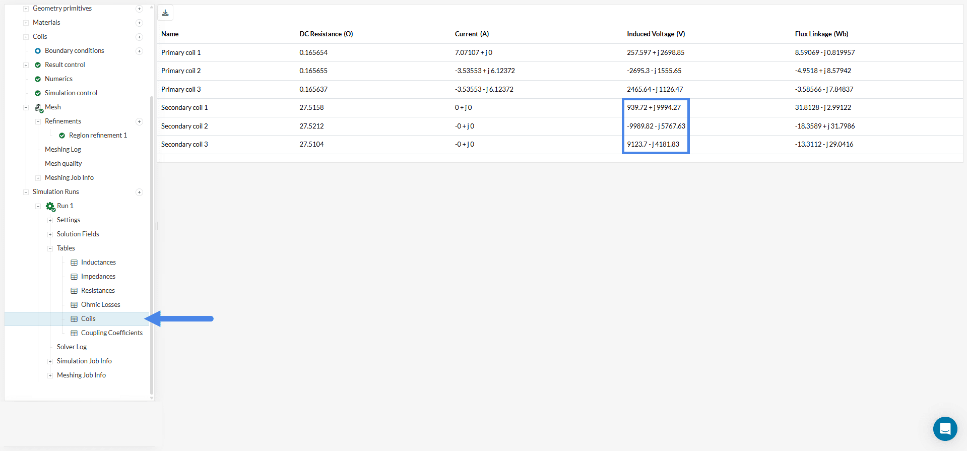
By expanding the tables under the completed run, you can check the induced voltage on the coils — a key result for evaluating the transformer’s efficiency.
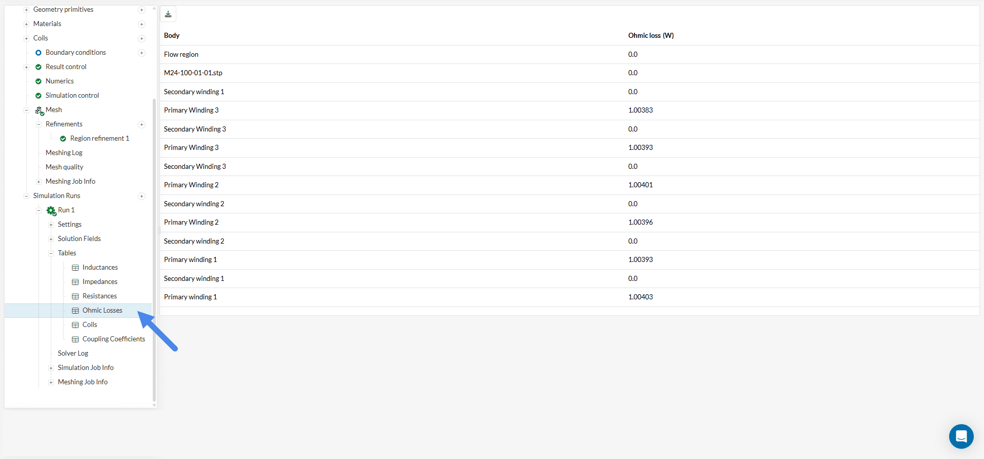
Ohmic losses can also be examined by selecting the corresponding table. These values are crucial for assessing the amount of Joule heating generated by the current flowing through the conductive materials.
The probe point results are particularly important in this simulation. As shown in Figure 29, the table displays the magnetic flux density at the core, obtained from the previously created result control item. In this case, the RMS magnetic flux density is 1.8064 \(T\).
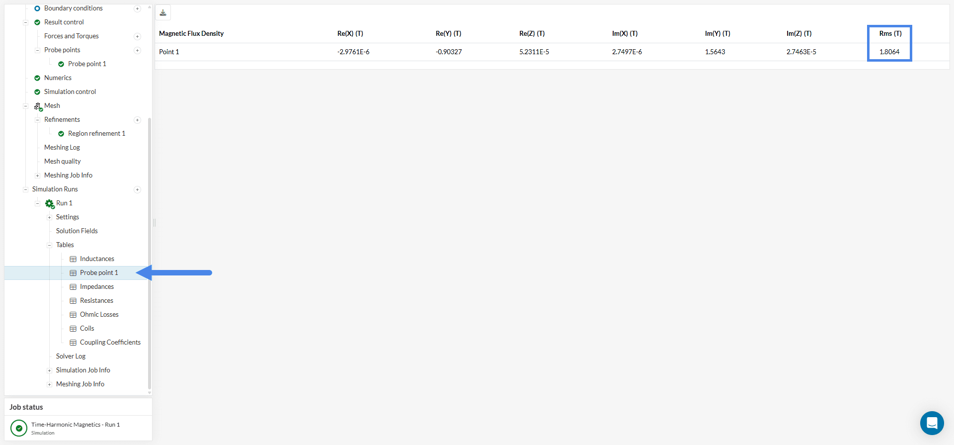
A comparison with Figure 17 shows that the core is approaching saturation, although it has not yet exceeded the saturation threshold.
Analyze your results further with the SimScale post-processor. Have a look at our post-processing guide to learn how to use the post-processor.
Note
If you have questions or suggestions, please reach out either via the forum or contact us directly.
Last updated: August 4th, 2025
We appreciate and value your feedback.
Sign up for SimScale
and start simulating now