Mesh Sensitivity Study for CFD Simulations

A question that commonly arises after running a CFD simulation is “Can I trust my results?” When it comes to increasing the confidence in the results, the practitioner can take advantage of several good practices—mesh sensitivity studies being one of the most important tools in this process.

Background

One of the requirements to run a CFD simulation is to split the computational domain into several discrete mesh cells. In a simulation, the governing flow equations and other models are applied and the results are calculated using the mesh as a base, and this process will originate spatial discretization errors.

By running a mesh sensitivity study, the user can have a better understanding of the spatial discretization errors and how much the mesh is affecting the solution. In an optimal scenario, as the cell size approaches zero, the spatial discretization error tends to zero as well.

From a practical perspective this means that when the user deems the results to be mesh independent, the results change very little with additional refinement.

Mesh Sensitivity Study

A mesh sensitivity study (also known as a mesh independence or mesh convergence study) consists of running the same simulation using grids with different resolutions and analyzing how much the converged solution changes with each mesh. For notes on how to assess the convergence of a simulation, please refer to this article.

Since CFD simulations can be very different in terms of physics and complexity, a concern is to obtain a generic workflow that can be used for a wide range of scenarios. One option is the Grid Convergence Index (GCI), proposed by Roache\(^{[1]}\). Interested readers can also find a detailed GCI description and formulation in this open NASA dedicated page on grid convergence.

Roache proposes workflows for unstructured grids, such as the standard tool, and structured grids, such as the hex-dominant and hex-dominant (parametric) tools. The following sections go through usual practices.

Standard Meshing Tool

When using the GCI approach, the user is advised to evenly refine/coarsen the domain for subsequent meshes. For unstructured meshes, such as those created with the standard tool, even refinement is not always possible to achieve.

With that in mind, Roache proposed an alternative approach for calculating the linear growth rate between adjacent 3D unstructured meshes:

$$r_{effective} = \big( \frac{N_1}{N_2} \big)^{1/3} \tag {1} $$

Where \(r_{effective}\) is the linear growth rate, \(N1\) is the cell count of the finer mesh, and \(N2\) is the cell count of the coarser mesh.

Below we have a set of three standard meshes with an \(r_{effective}\) of 1.26 between them:

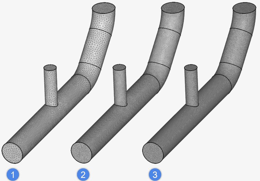
One could use the above set of meshes as a starting point for a sensitivity study.

Hex-Dominant (Parametric)

For structured meshes, such as the hex-dominant parametric tool, it’s easier to ensure an even refinement throughout the entire domain. The logic is to start with a base mesh and refine (or coarsen it) by adjusting the Bounding box resolution by applying the growth rate.

As an example, the mesh below is the base mesh of our study, with a Bounding box resolution of 15 cells in x, 146 cells in y, and 45 cells in z:

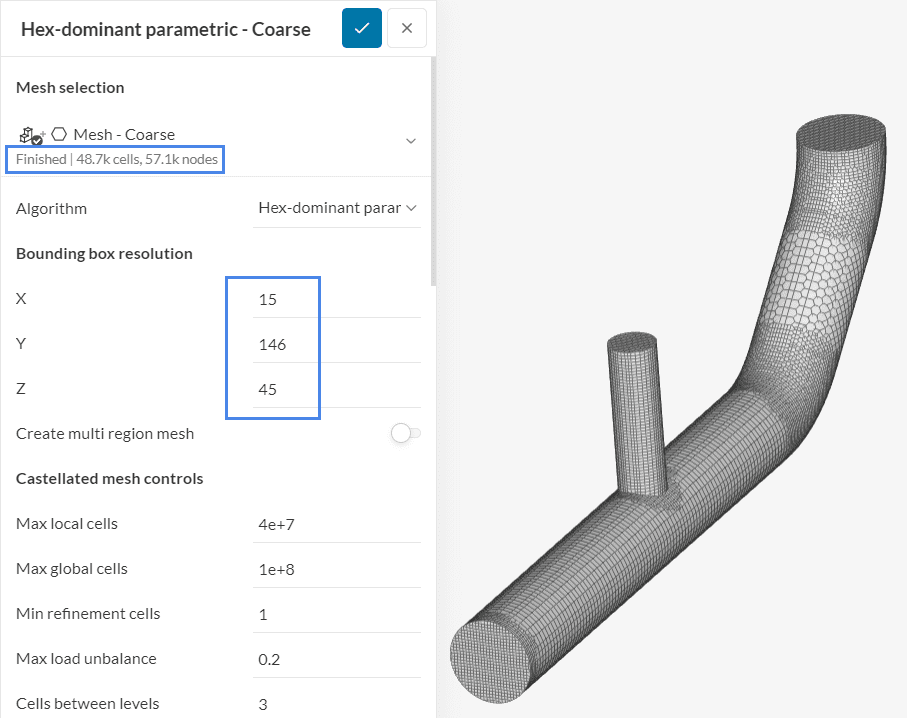
This initial mesh has roughly 49 thousand cells. By multiplying the Bounding box resolution by 1.26 and rounding up the values, the mesh is evenly refined in the entire domain:

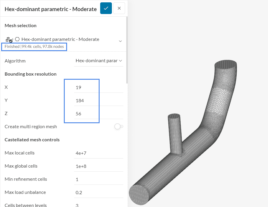
Since the meshing operation is an iterative process, the number of cells won’t be exactly twice as much. The user may further adjust the bounding box resolution if necessary. Finally, by multiplying the bounding box resolution by 1.26 again, we may obtain the fine mesh:

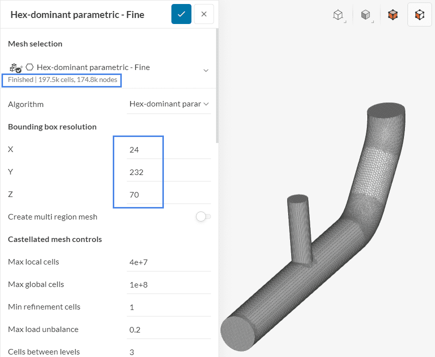
With this set of three meshes, one could run a sensitivity study.

Expected Results

When the asymptotic convergence region is achieved, the solution will vary a small amount between the moderate and fine meshes. Following the GCI formulation\(^1\), it is possible to obtain extra insights, such as an extrapolation of the asymptotic value for a cell size approaching zero.

For example, after running the pipe simulation for the three meshes and monitoring the parameter of interest (delta pressure) via result controls, we may find the following solution set:

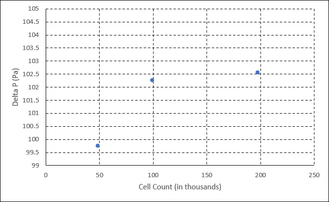
Despite the cell count doubling for each mesh, the parameter of interest shifts very little between subsequent meshes. It is valuable for the practitioner to understand how much the solution varies for different mesh sizes, so they can apply adequate refinement for their studies.

References

- P. J. Roache. “Perspective: A Method for Uniform Reporting of Grid Refinement Studies”. J. Fluids Eng. Sep 1994, 116(3): 405-413 (9 pages).
- NASA. Examining Spatial (Grid) Convergence.
- Richardson Lewis Fry and Gaunt J. Arthur 1927. VIII. The deferred approach to the limit. Philosophical Transactions of the Royal Society of London.