Tutorial: Electromagnetics Simulation on a Linear Pushing Solenoid
This tutorial showcases how to use SimScale to run an electromagnetics simulation on a Linear Pushing Solenoid, where the objective is to achieve the linear pushing force of the solenoid to see how it works.
Overview
This tutorial teaches how to:
- Setup and run an electromagnetics simulation;
- Create an external flow region;
- Assign multiple materials, and other properties to the simulation;
- Mesh with the automatic standard meshing algorithm.
We are following the typical SimScale workflow:
- Prepare the CAD model for the simulation;
- Set up the simulation;
- Create the mesh;
- Run the simulation and analyze the results.
1. Prepare the CAD Model and Select the Analysis Type
To begin, click on the button below. It will copy the tutorial project containing the geometry into your Workbench.
The following picture demonstrates what is visible after importing the tutorial project.
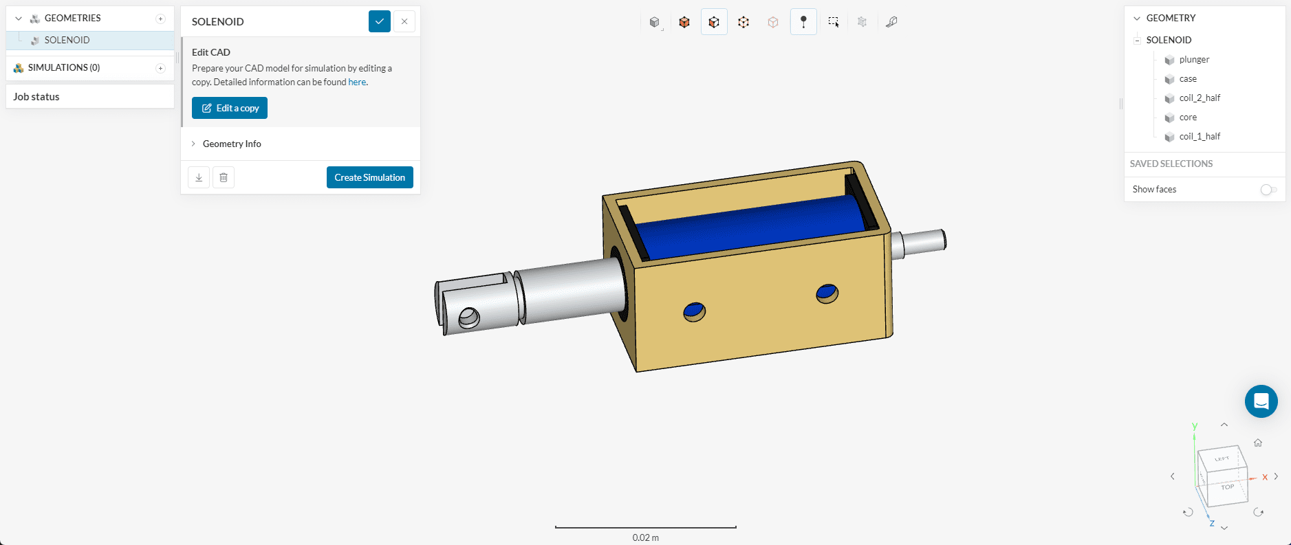
The geometry consists of a linear actuating solenoid. It consists of multiple parts as can be observed in the scene tree.
1.1 Geometry Preparation
The geometry for this tutorial is not ready for electromagnetic simulations. It contains multiple solid parts, however we also need a single flow volume region for setting up the simulation.
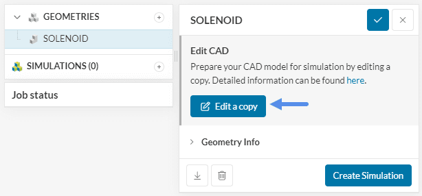
To create a flow volume click on the ‘Edit a copy’ icon.
Follow the steps below as shown in Figure 4 to create the external flow volume.
- Select the external flow volume tool
- Apply with the default Box dimensions.
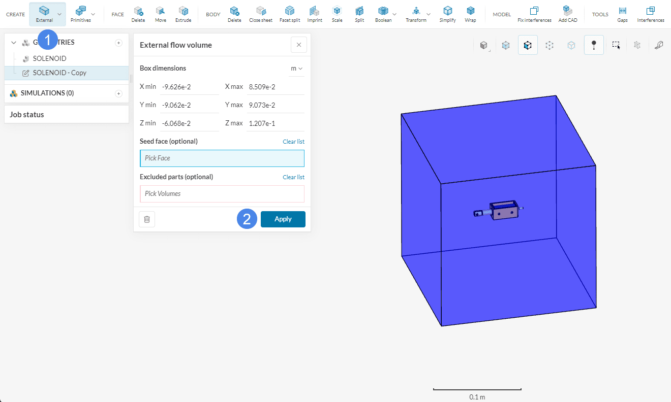
Notice that there is a new volume entity called Flow region under the parts list at the very end (see Figure 5). Use the ‘Save’ button to save this new geometry in the Workbench.
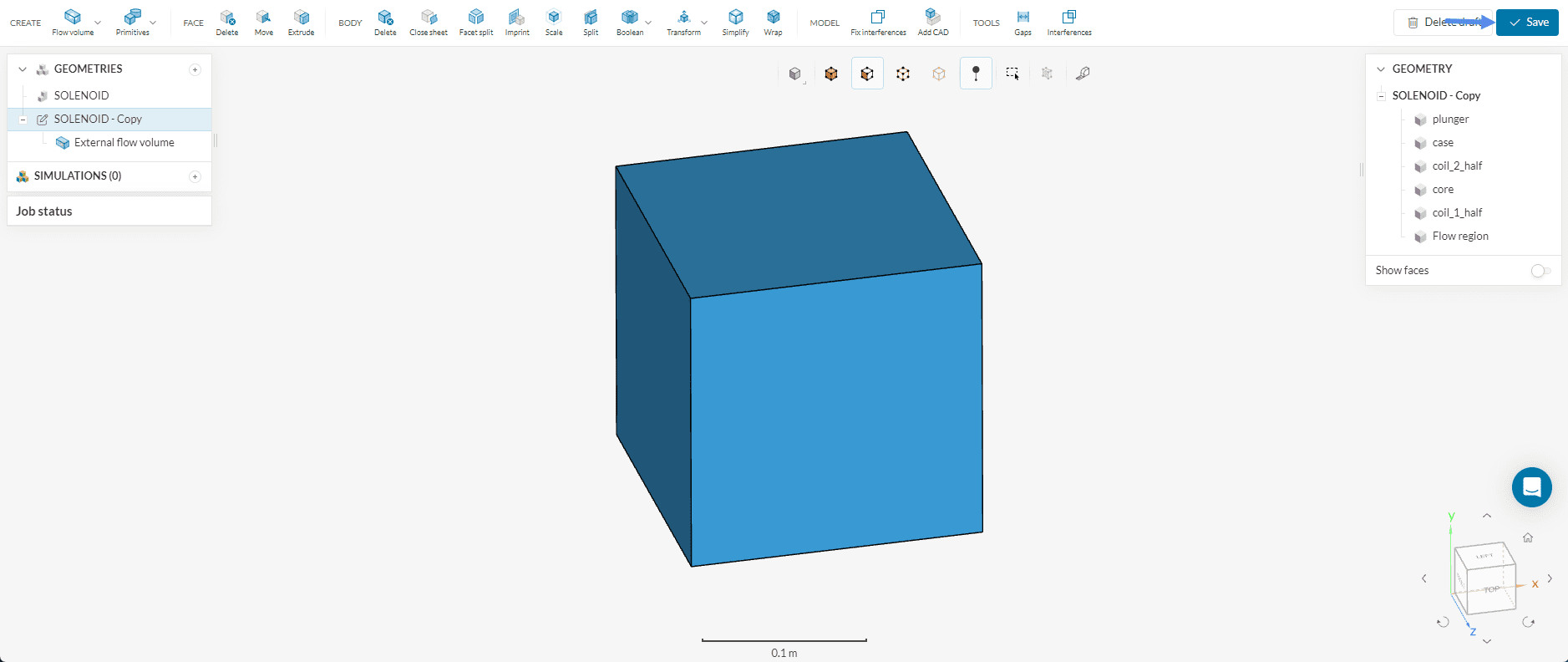
The modified geometry (with the Flow region) will appear under Geometries as a copy of the original solenoid geometry.
1.2 Create the Simulation
Click on the new geometry ‘Copy of Magnetic Lifting Machine’, rename it to “Flow Region SOLENOID” and hit the ‘Create Simulation’ button, to start the simulation setup process.
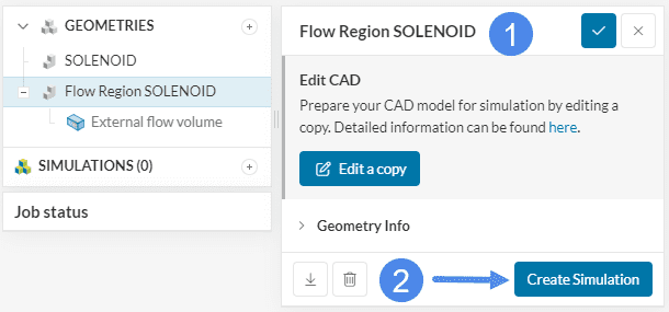
This will open the simulation type selection widget:
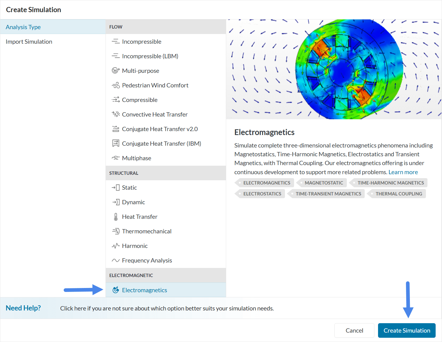
Choose ‘Electromagnetics‘ as the analysis type and ‘Create Simulation’.
At this point, the simulation tree will be visible in the left-hand side panel.
2. Pre-Processing: Setting up the Simulation
2.1 Define Materials
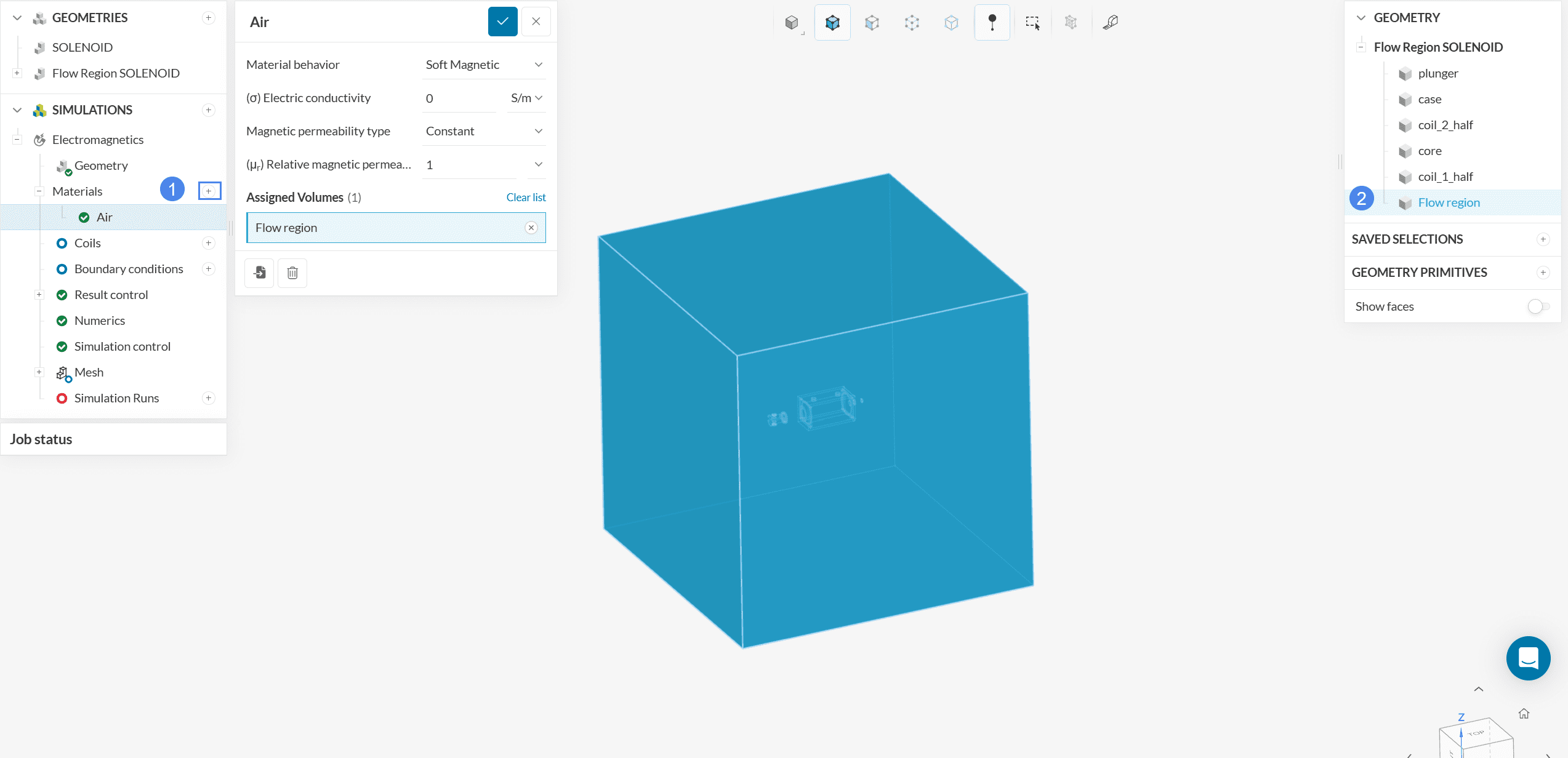
This simulation will begin with air present in the flow region. Then we will assign copper, plastic, and metal to the solid bodies. Therefore, this simulation will use four materials. To start assigning, click on the ‘+ button’ next to Materials. In doing so, the SimScale fluid material library opens, as shown in the figure below:
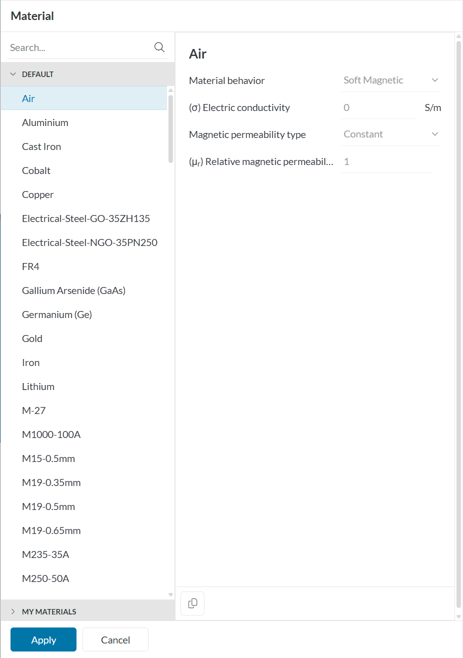
Select ‘Air‘ and click ‘Apply’. This means air will be recognized by the flow region throughout the simulation. Keep the default values, and assign the entire Flow region to it (if not already by default).
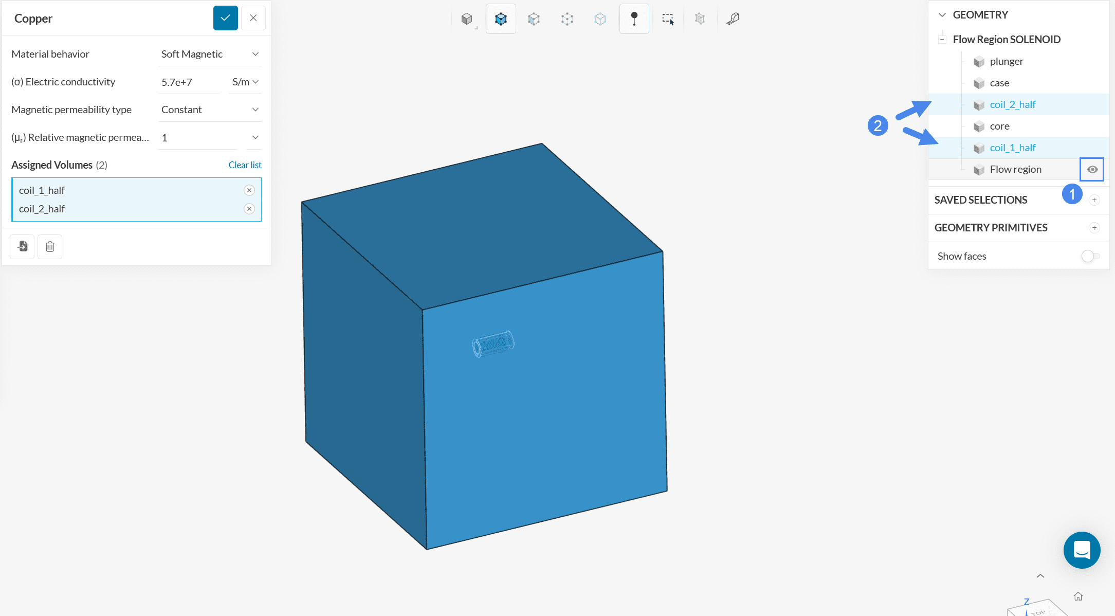
Repeat the same procedure for the material ‘Copper’ and assign it to the coils. Hide the Flow region such that the coils are visible Figure 10. Now assign the material to ‘coil_1_half’ and ‘coil_2_half’.
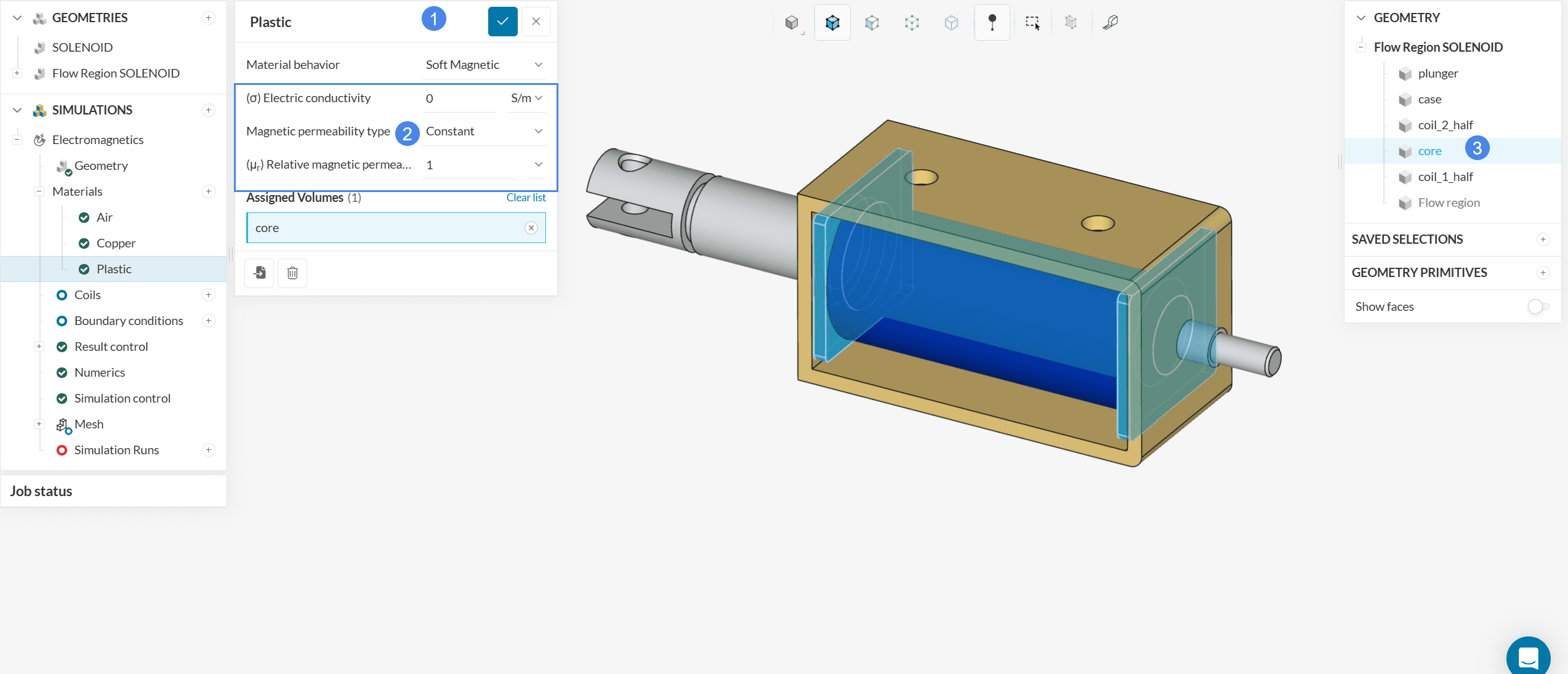
For the plastic core, a custom material needs to be created. To do this create a new material and select ‘Steel’. Change the name of the material to ‘Plastic’ and adjust the Electric conductivity to ‘0’ \(S/m)\. Lastly, assign the core to the newly created material.
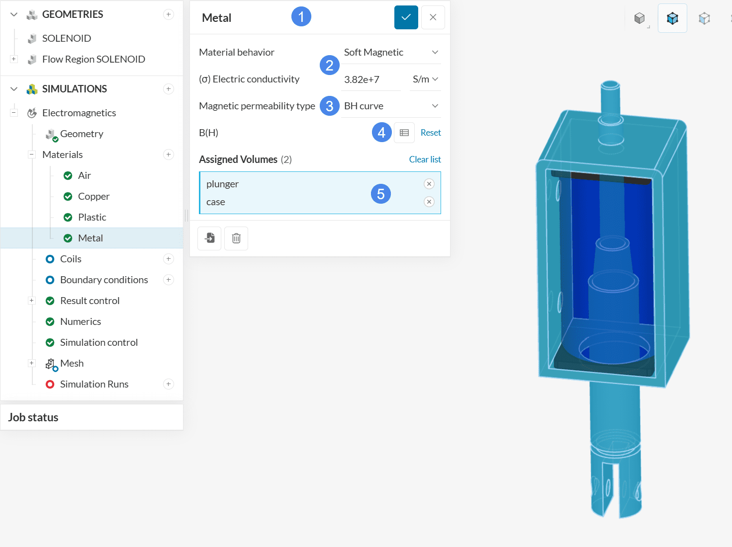
Lastly, repeat the process to create a new custom material for the metal of the case and the plunger. Again create a steel material and adjust the name to ‘Metal’. Let the behavior be Soft Magnetic. Adjust the Electric conductivity to ‘3.82e+7’ \(S/m)\. To accurately model the magnetic permeability, change the type to ‘Nonlinear Isotropic’, and assign the following B/H Curve. As a last step assign the case and the plunger to the metal material.
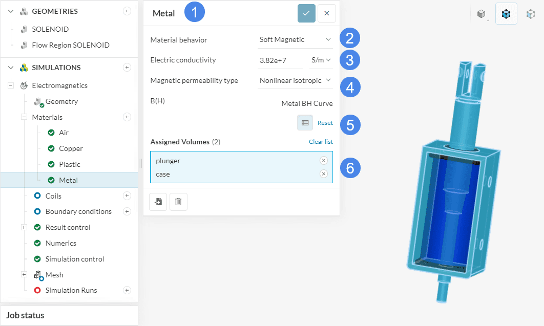
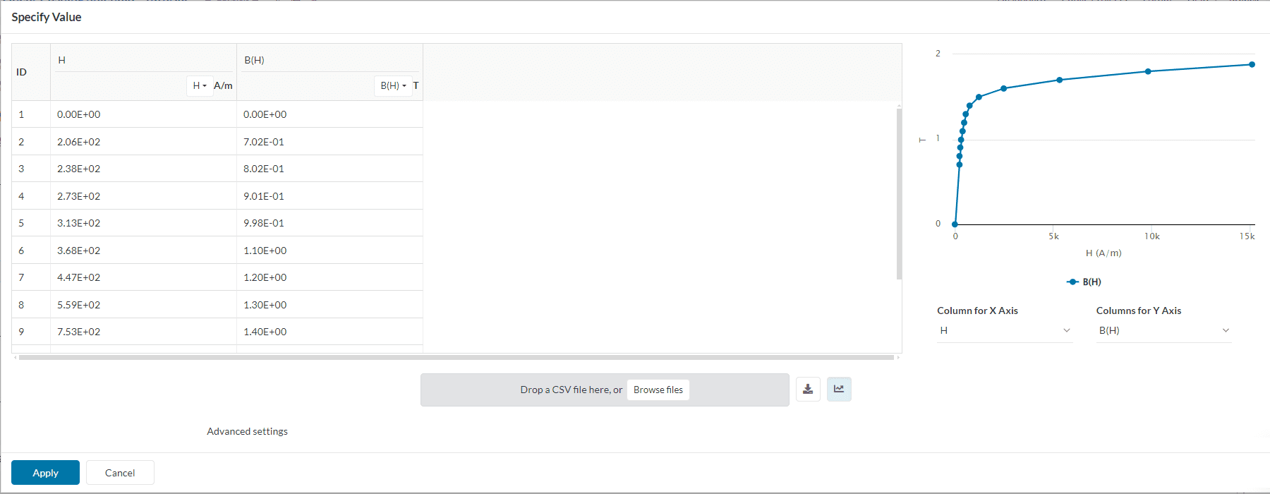
Please find the B/H curve for the metal material below. Figure 13 shows the assigned material table as well as the B/H curve.
2.2 Assign the Coils
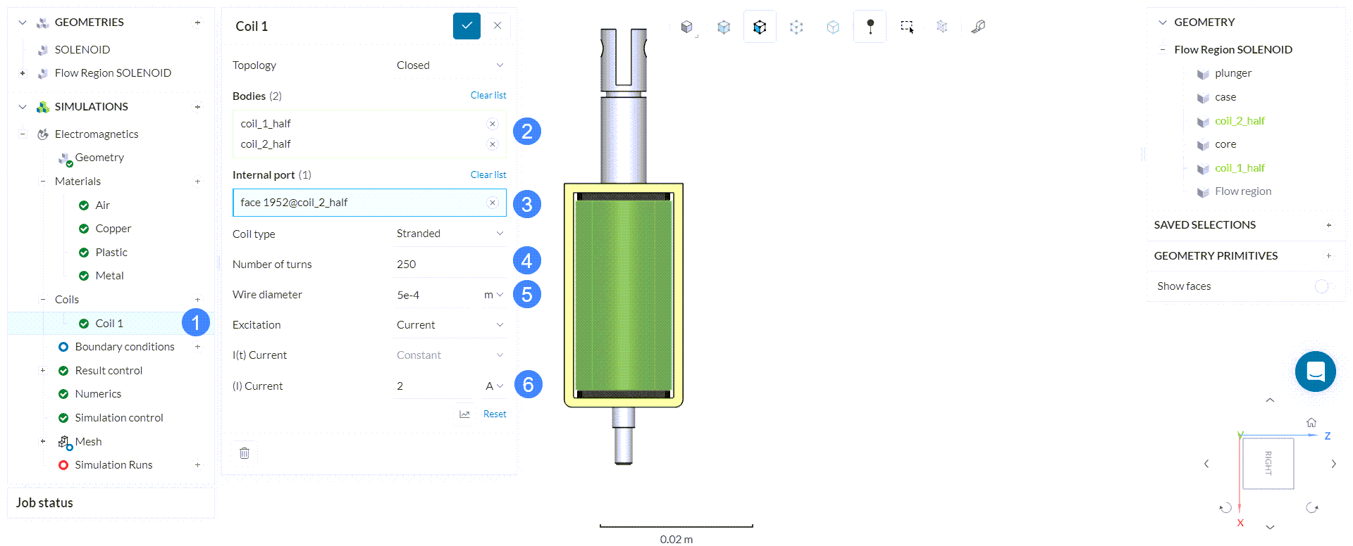
Under Coils in the simulation tree, create a new closed coil. To specify the internal port of the coil it has been cut into two halves, thus both halves are assigned in a single coil setting. Assign the ‘Coil_1_half’ and ‘Coil_2_half’ to bodies. Please select an inner face and change the respective values as shown in Figure 14. Please set the values for Topology, Number of turns, Wire diameters, and (I) Current.
Tool Tip
By right-clicking on the inside face of the two coils you can use the assign other option to select the hidden inside face of the coil without the need to hide one of the coil parts. More tips and tricks on the selection tools within SimScale can be found here.
2.3 Assign the Boundary Conditions
There is no need to assign boundary conditions for this simulation.
2.4 Result Control
Result control allows you to observe the convergence behavior globally as well as at specific locations in the model during the calculation process. Hence, it is an important indicator of the simulation quality and the reliability of the results. Remember to toggle on ‘Calculate Inductances’ under Result control.
a. Forces and Torques
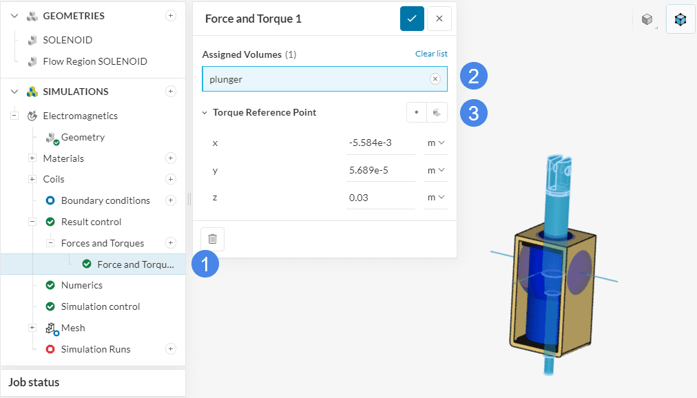
For this simulation, set a ‘Forces and torques’ control on the plunger. Click on the ‘+’ icon under Result control> Forces and torques to open the settings panel. After assigning the plunger volume to the result control, select the ‘Pick center of the current selection’ tool to set the Torque Reference Point.
2.5 Numerics and Simulation Control
The Numerics and Simulation control for this simulation, are optimised with their default values and need not be altered.
3. Mesh
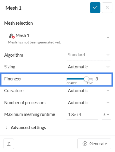
To create the mesh, we recommend using the Automatic mesh algorithm, which is a good choice in general as it is quite automated and delivers good results for most geometries.
In this tutorial, a mesh fineness level of 8 will be used. If you wish to undertake a mesh refinement study, you can increase the fineness of the mesh by sliding the Fineness slider to higher refinement levels or using custom refinements.
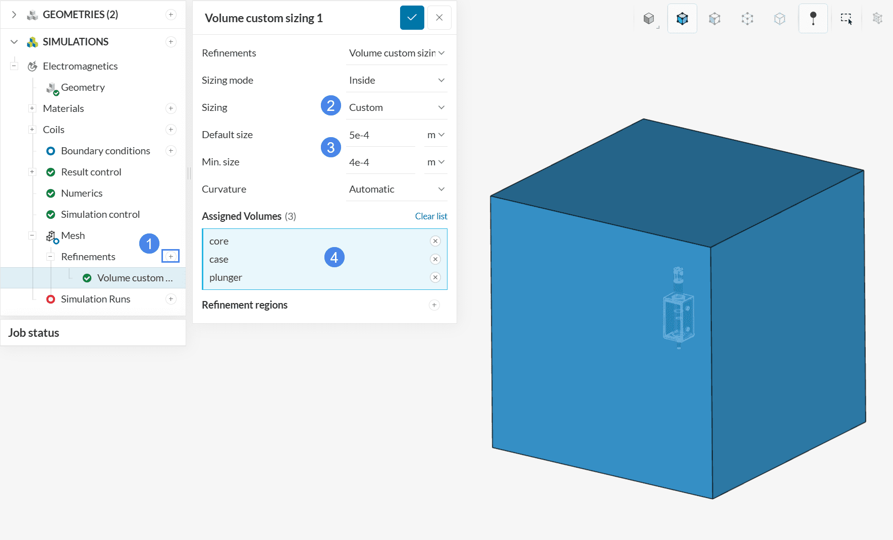
In addition to the mesh fineness of level 8, the plunger, case, and core, will have a Volume custom sizing refinement with a Default size of ‘5e-4’ \(m\) and a Min. size of ‘4e-4’ \(m\). To do this create a new refinement and assign the parts as shown in Figure 17.
Did you know?
The automesher creates a body-fitted mesh which captures most regions of interest using physics based meshing.
4. Start the Simulation
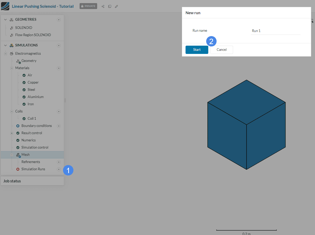
Now you can start the simulation. Click on the ‘+’ icon next to Simulation Runs. This opens up a dialogue box where you can name your run and ‘Start’ the simulation.
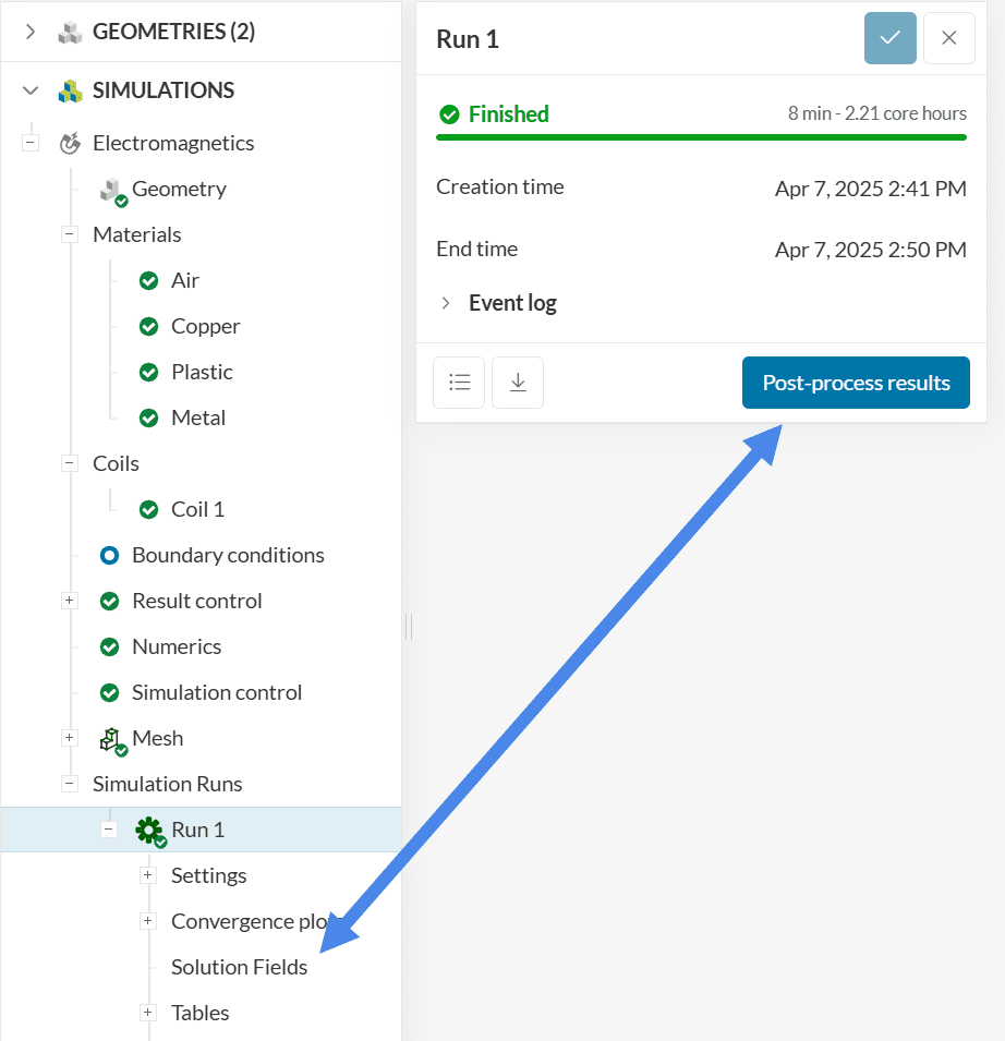
While the results are being calculated you can already have a look at the intermediate results in the post-processor by clicking on ‘Solution Fields’ or ‘Post-process results’. They are being updated in real time! Once finished access the online post-processor as indicated in Figure 19.
5. Post-Processing
5.1 Solution Field
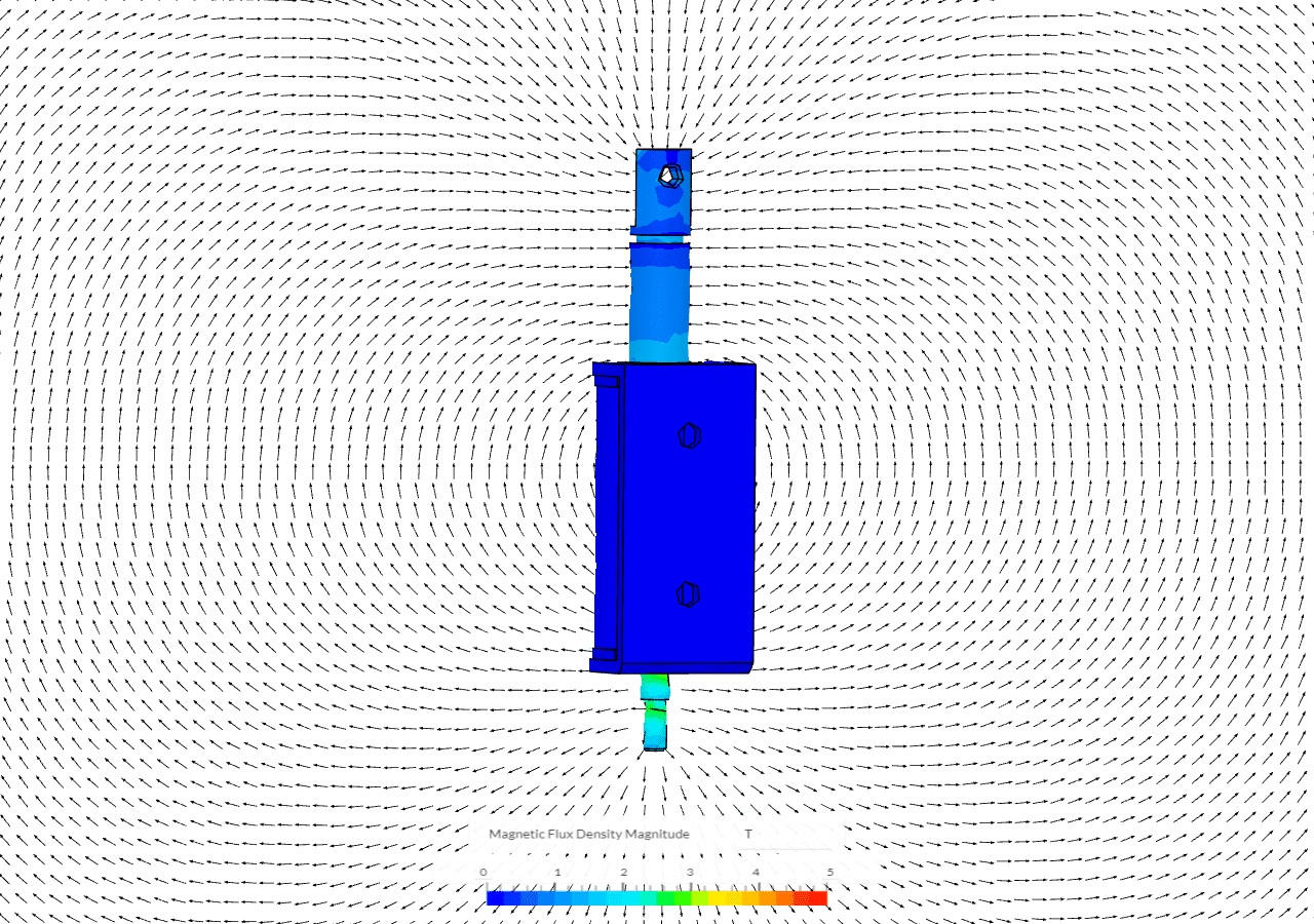
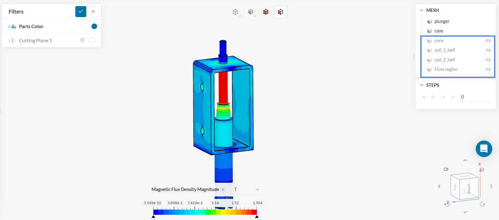
Once inside the post-processor, you can first investigate the magnetic flux density. To do this toggle the cutting plane off and hide the Flow Region, coil_1_half, coil_2_half, as well as the core by clicking on the eye icon.
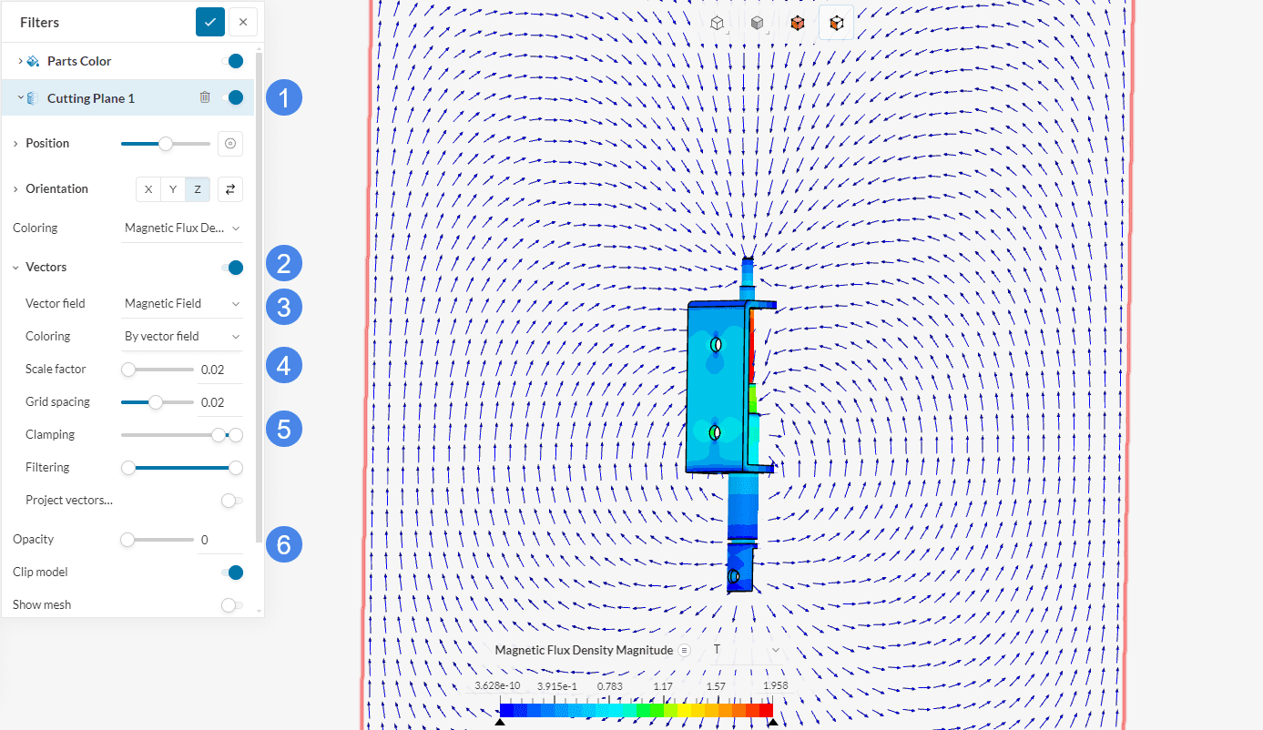
In order to visualize the magnetic field around the part, turn the visualization of the cutting plane back on. Here activate the vectors option and switch the vector field to the ‘Magnetic field’. Next, change the scale factor to ‘0.02’ and adjust the lower slider for clamping to 90 %. Lastly, turn the opacity of the cutting plane to ‘0’ so that only the vectors are left visible.
More spaced-out lines signify lower densities. The direction of the lines illustrates the path a positive charge would take. The continuous nature of these lines indicates the uninterrupted flow of current.
5.2 Forces and Torques on the Load
The Forces and torques results are of particular interest in the simulation. From the earlier-created result control item, the forces and moments acting on the plunger can be seen in the table in Figure 22. In this case, the axial force on the plunger is 0.0407 \(N\).
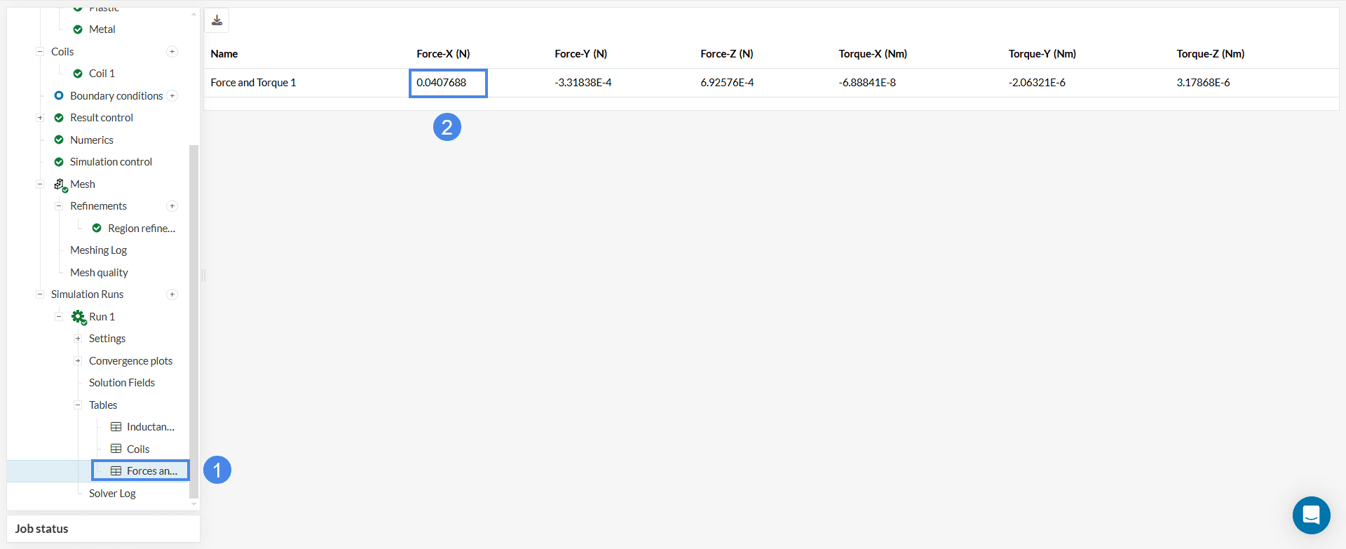
Numerical Noise
The quantity of interest is the X-component of force. Rerunning the simulation might result into different values for the Y and Z component which represent numerical noise due to cancellation errors and the values should be close to 0 due to symmetry.
Analyze your results further with the SimScale post-processor. Have a look at our post-processing guide to learn how to use the post-processor.
Note
If you have questions or suggestions, please reach out either via the forum or contact us directly.
Last updated: November 7th, 2025
Did this article solve your issue?
How can we do better?
We appreciate and value your feedback.


