What is Cavitation?
Cavitation happens when the local static pressure falls below the vapor pressure of the working liquid, causing the liquid to evaporate into vapor bubbles. These bubbles get trapped in small pockets and travel downstream. When the local pressure rises again, these vapor pockets implode, causing localized shock waves which can damage the pump equipment and lead to excessive noise and vibrations.
Simply stated, cavitation is a detrimental phenomenon caused by the rapid formation and collapse of vapor bubbles in a pump. Let’s first understand the causes of cavitation before diving deeper into methods used to spot and mitigate it.
What Causes Cavitation?
Physics of Phase Change and Equilibrium
Cavitation is governed by the physics of phase transition and equilibrium. The current discussion is presented for water, however, the same principles can be extended to other pure substances as well.
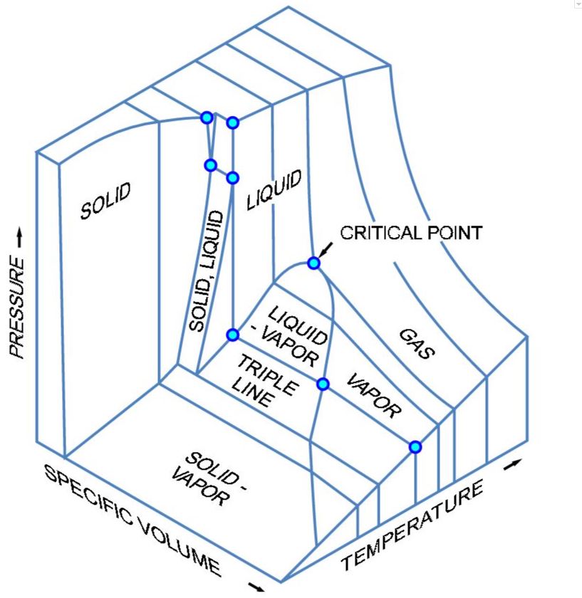
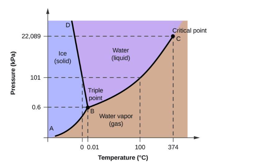
The boiling point of water is 373 K, which means that at 373 K and atmospheric pressure, there is a liquid-vapor equilibrium for water. In fact, we can find a continuous range of temperatures as the pressure changes for which such an equilibrium exists. This phase equilibrium is visualized on a Pressure-Temperature (P-T) diagram, as shown in Figure 2. The projection of the surface on the P-T plane will give us the P-T diagram, as shown in Figure 3.
Phase Change and Cavitation
Upstream of the pump inlet, the static pressure of the flow drops due to frictional losses and acceleration. As the fluid flows downstream, the pressure further drops due to blade thickness and incidence angle.
The process is isothermal i.e. the temperature of the fluid does not change. In Figure 3, the process would follow a vertical line from top to bottom, starting from the liquid region between B and C. The endpoints are determined by the starting pressure and subsequent pressure drop. If the pressure drops enough such that the endpoint crosses the liquid-vapor line, then cavitation occurs.
Cavitation and Net Positive Suction Head
Cavitation is usually defined in terms of the Net Positive Suction Head Available \(NPSH_a\) and the Net Positive Suction Head Required \(NPSH_r\) for the pump to operate free of cavitation. \(NPSH_a\) is defined as:
$$NPSH_a = \frac{p_s – p_v}{\rho g} + \frac{C_s^2}{2g}\tag{1}$$
| Symbols | Meaning |
| \(p_s\) | static pressure at the pump inlet |
| \(p_v\) | liquid vapor pressure at the given temperature |
| \(\rho\) | fluid density |
| \(g\) | acceleration due to gravity |
| \(C_s\) | flow speed at the pump inlet |
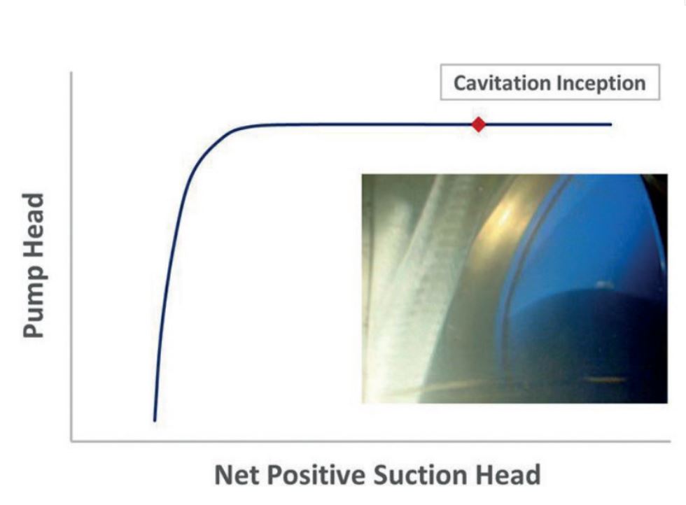
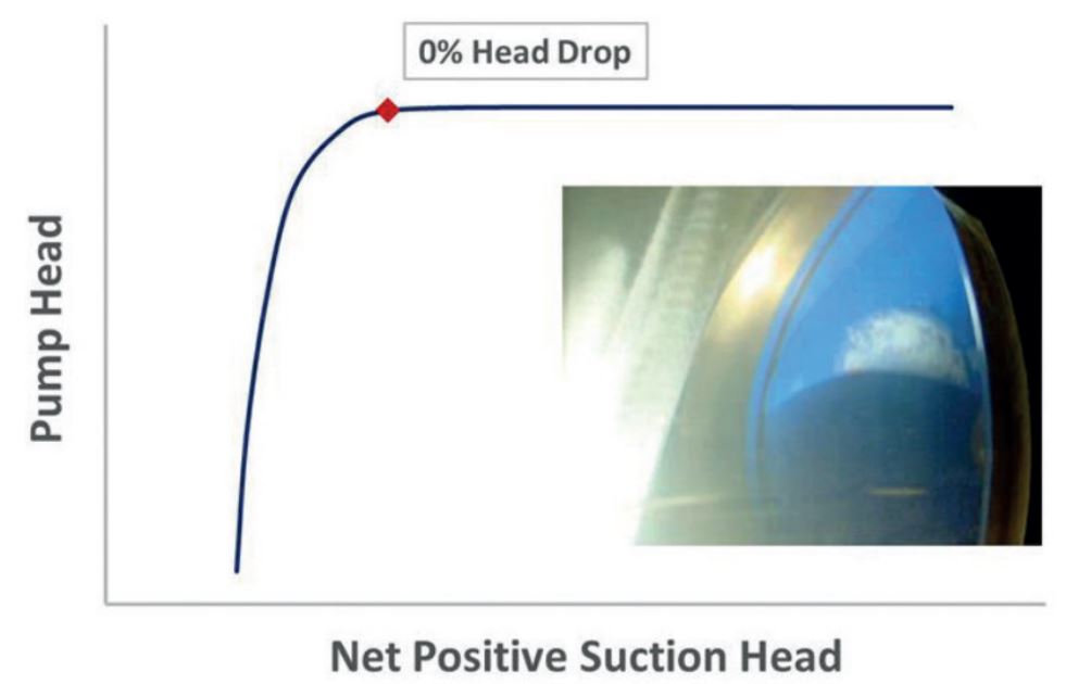
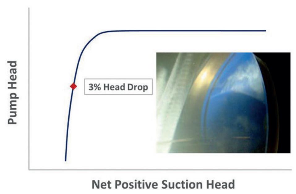
The exact value of the pressure at which cavitation starts is difficult to predict and depends on a lot of factors. The Net Positive Suction Head for which the pump head drops by 3% ((NPSH_3)) is much easier to measure and is the most commonly used term in pump specification to indicate the minimum recommended (NSPH) to avoid cavitation.
Why is Cavitation Bad?
One of the main effects of cavitation is the drop in pump performance. As the cavitation fraction in the flow increases, the head developed by the pump decreases, as shown in Figures 5, 6, and 7.
Cavitation also causes additional noise and vibrations due to the high-pressure pulses generated from the implosion of the cavitation bubbles. These implosions cause broad-spectrum high-frequency fluid-borne noise in the kHz range.
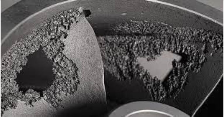
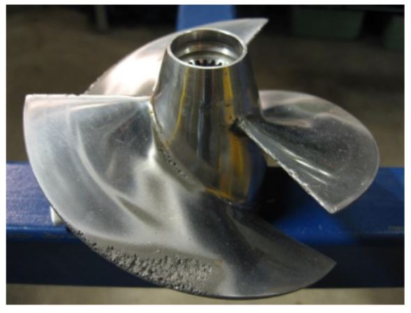
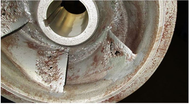
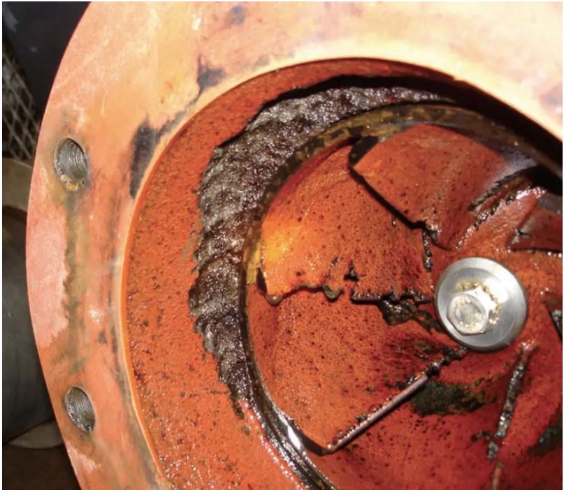
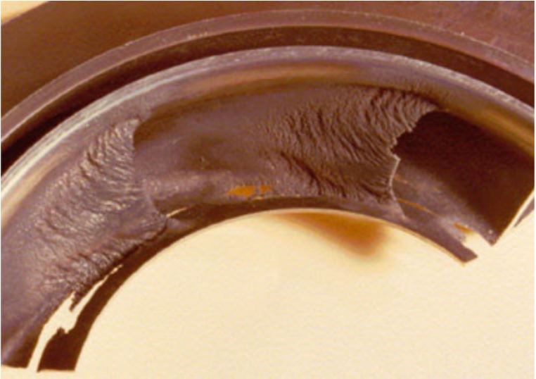
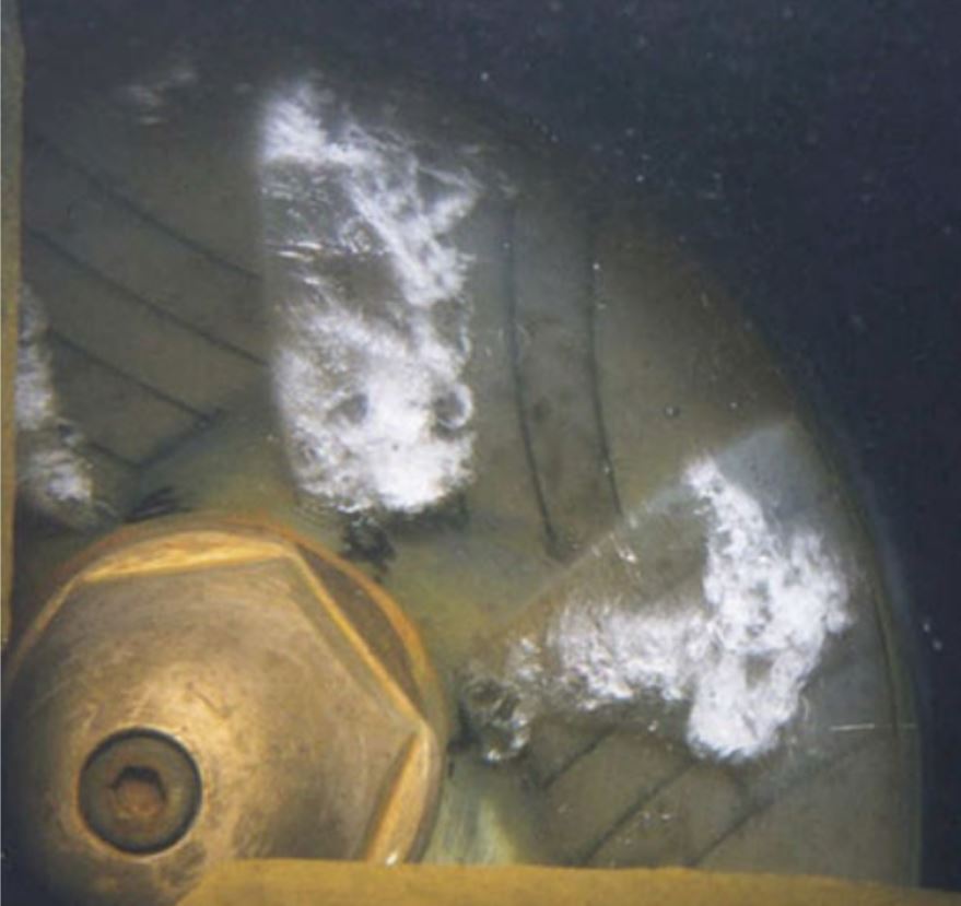
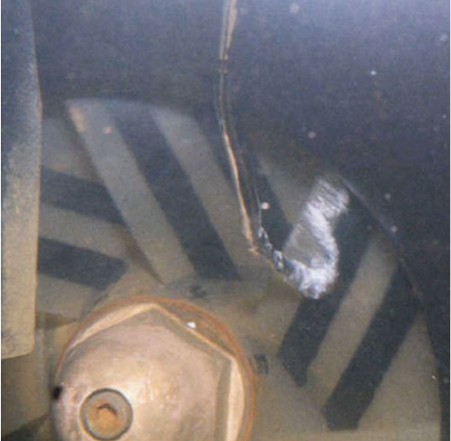
Cavitation may also cause structural damages like the ones shown in Figures 9 – 12.
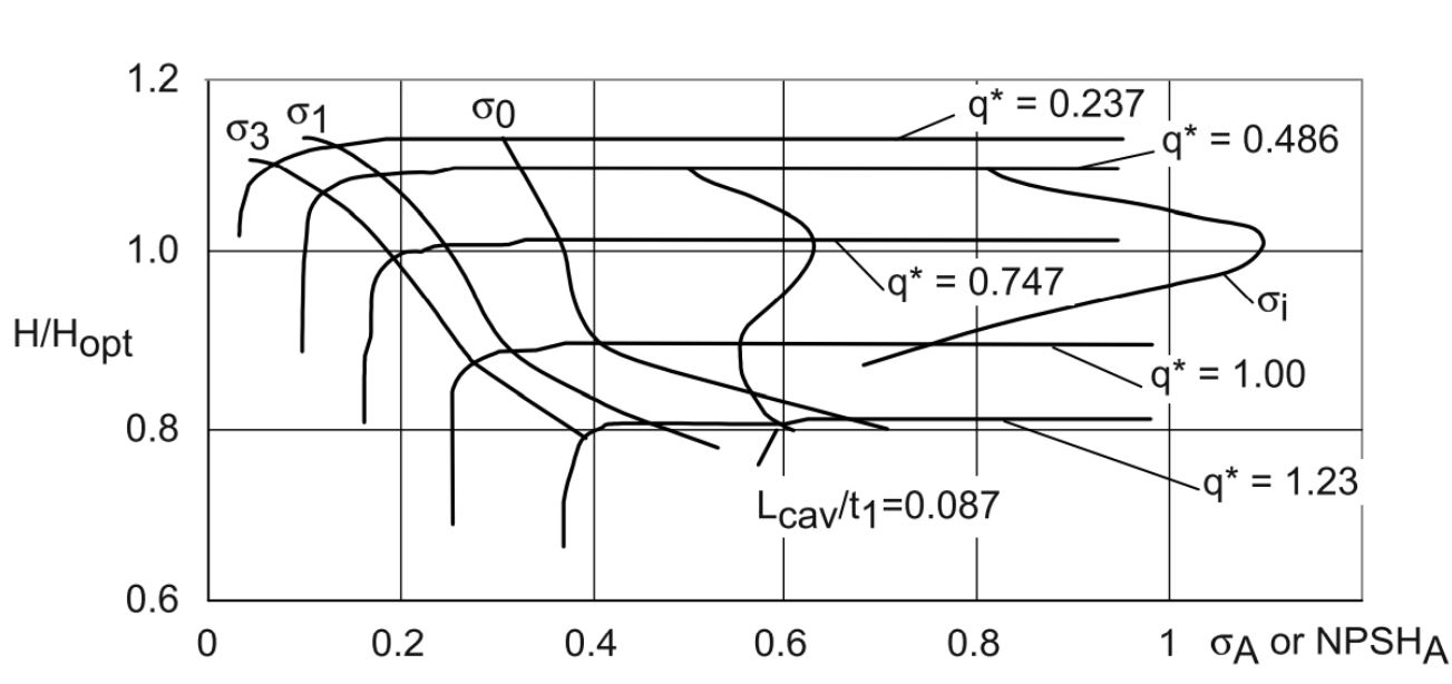
Complete Head drop charts for different mass flow rates are shown in Figure 8. Here, both flow rates and head developed have been normalized using the design point head developed and design point mass flow rate. Additional curves are added to show cavitation inception \(\sigma_i\), beginning of head drop \(\sigma_o\) , 1% head drop \(\sigma_1\), and 3% head drop \(\sigma_3\). Here, \(\sigma_x\) is defined as follows:
$$\sigma_x = \frac{2g NPSH_x}{u_{1a}^2} \tag{2}$$
| Symbols | Meaning |
| \(NPSH_x\) | Net Positive Suction Head |
| \(g\) | Acceleration due to gravity |
| \(u_{1a}\) | Inlet blade speed at the shroud |
Where Does Cavitation Occur?
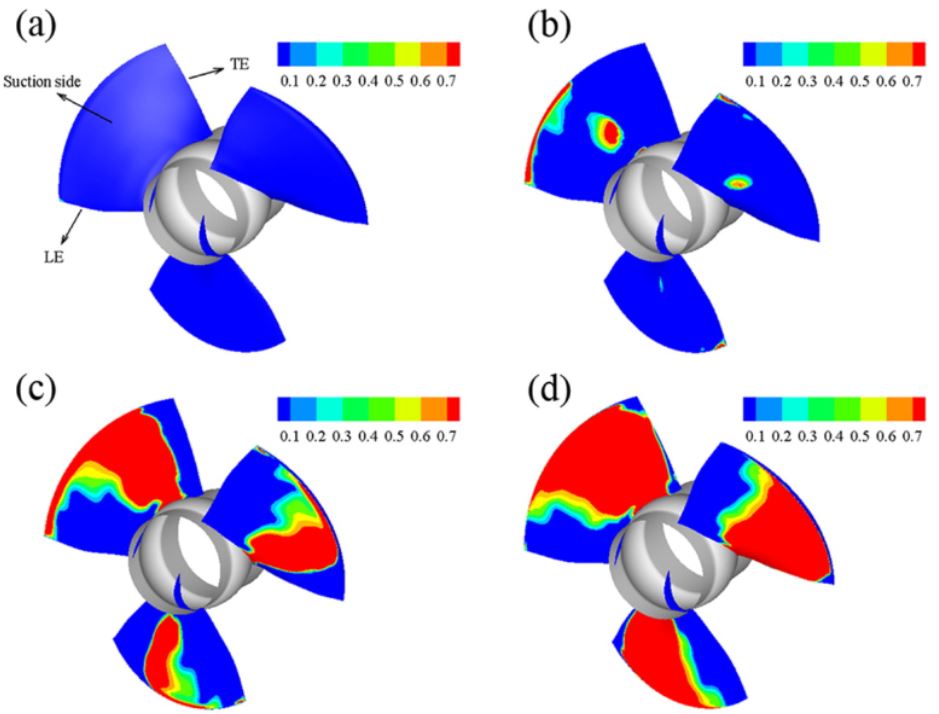
Cavitation is a very common occurrence and can happen within any pump working at unsuitable inlet pressures or badly designed components. For centrifugal or mixed flow pumps, cavitation normally happens at the inlet of an impeller or inducer. For axial flow pumps, cavitation also occurs close to the inlet at the blade tip close to the shroud or sometimes at the middle of the blade suction side as shown in Figure 13.
How to Avoid Cavitation?
The methods of avoiding cavitation depend upon the type, location, and intensity of the cavitation. Some of the suggested causes and the remedies based on the cavitation damage pattern or the cavity location are as follows\(^7\):
| Cavitation pattern location/characteristics | Causes | Solutions |
| Attached cavity and/or damage observed on the suction side close to the leading edge. | Incidence angle too large, unfavorable leading edge profile. | There is a mismatch between the flow angle and the blade angle, so increasing the flow rate, introducing pre-rotation in the flow, or increasing the axial flow speed using inlet rings will reduce cavitation. |
| Long, thick cavity along with vortex shedding on the suction side. Damage observed on the suction side within the impeller channel far from the leading edge. | Suction head available is too low, incidence angle too large. | Increase the flow speed by increasing the flow rate, drill holes on the blade to allow flow from suction to pressure side. |
| Attached cavity on the pressure side, damage near the leading edge close to the shroud. | Unfavorable leading edge profile, excessive flow rates. | Reduce the flow rate, cut back blade and profile on the pressure surface. |
| Cavity cloud in the impeller channel due to flow recirculation. | Intensive flow deceleration, due to large impeller diameter, low flow rate, and high blade angles where higher angle implies blades being more meriodinal. | Increase flow rate, improve leading edge profile by grinding. |
| Gap cavitation in unshrouded impellers. | High Blade loading. | Rounding of the blade edge on pressure surface. |
General Principles for Reducing Cavitation and Its Effect
In addition to the solution given above, all kinds of cavitation-related damages can be reduced by using one or more of the ways stated below:
- Increasing the inlet pressure is always the best solution. Sufficient inlet pressure can reduce or even eliminate cavitation, but doing so is not always possible.
- In high-speed applications, where increasing inlet pressure is not possible, an inducer is used instead. The inducer can handle a certain amount of cavitation and by the time the flow reaches the impeller inlet the cavitation bubbles are usually suppressed and inlet pressure is sufficiently increased to avoid major cavitation within the main impeller.
- Using a more cavitation-resistant material like high-strength nickel chromium steel or Titanium or Inconel for very high-speed mass critical applications like the ones expected to find in a rocket turbopump\(^7\).
How to Predict Cavitation?
In general, it is very difficult to predict cavitation using analytical techniques. It is much easier to check for cavitation using experiments. However, experiments are usually expensive and time-consuming. Moreover, it would benefit pump customers if pumps are designed to prevent cavitation, rather than troubleshoot performance issues after the pump is in operation.
CFD simulations can add valuable insights by enabling design space exploration to develop pump systems with minimized cavitation, while also being valuable as a tool for aftermarket repairs.
Pump Inlet Design for Minimizing Cavitation
Here, we describe semi-empirical-analytical ways of calculating \(NPSH\) for a pump, which can be used to assess if the pump inlet pressure is sufficient to prevent cavitation or not. The relations presented here are from Gülich\(^7\) and are valid for centrifugal pumps as well as mixed flow pumps to some extent. Cavitation happens in regions of local pressure minima, which in turn are created due to local excessive flow speed around the blade leading edges. Equation 3 can be used for capturing these effects:
$$NPSH_3 = \lambda_c\frac{c_{1m}^2}{2 g} + \lambda_w\frac{w_1^2}{2 g}\tag{3}$$
| Symbols | Meaning |
| \(\lambda_c\) | coefficient accounting for flow acceleration and losses at the inlet |
| \(\lambda_w\) | coefficient denoting the low-pressure peaks at the blade inlet |
| \(w_1\) | relative flow speed at the impeller blade inlet at the shroud |
| \(c_{1m}\) | meridional component of the absolute flow speed at the impeller blade inlet |
| \(g\) | acceleration due to gravity |
The value of \(\lambda_c\) can be taken to be ~1.1 for axial flow inlet and 1.2 to 1.35 for radial inflow casing. Since the absolute flow speed is usually much smaller than the relative flow speed in a pump, the value of \(\lambda_w\) is much more significant. The value of \(\lambda_w\) depends upon numerous other parameters including inlet flow velocity profile, impeller, collector, and seal design. Roughly, the value of \(\lambda_w\) can be considered anywhere between 0.1 to 0.3 for impellers and 0.03 to 0.06 for inducers as a first approximation for pumps operating close to design flow rates. If \(\lambda_c\) and \(\lambda_w\) are assumed to be independent of inlet diameter, which is not strictly accurate, especially for \(\lambda_w\), an optimized inlet diameter can be obtained for which \(NPSH_3\) is maximum using the following equations:
$$c_{1m} = \frac{4Q}{\pi(d_1^2 – d_n^2)}\tag{4}$$
$$w_1^2 = c_{1m}^2+\left(u_{1a}-\frac{c_{1m}}{\tan{\alpha_1}}\right)^2\tag{5}$$
$$ u_{1a} = \frac{\pi d_1 n}{60}\tag{6}$$
| Symbols | Meaning |
| \(c_{1m}\) | meridional component of the absolute flow speed at the impeller blade inlet |
| \(Q\) | volume flow rate |
| \(n\) | blade rotation speed in rpm |
| \(\alpha_1\) | the angle between the direction of circumferential and absolute velocity at the shroud |
| \(w_1\) | relative flow speed at the impeller blade inlet |
| \(u_{1a}\) | impeller inlet blade speed at the shroud |
| \(d_1\) | impeller/inducer inlet diameter |
| \(d_n\) | impeller/inducer hub diameter |
Substituting Equations 4-6 in Equation 3 for \(NPSH_3\) and differentiating with respect to \(d_1\) and equating it to 0 gives the following result. The equation is also assuming that \(d_n\) is independent of \(d_1\) which is usually the case as \(d_n\) is dictated by the mechanical properties of the material.
$$ d_1 = \left(d_n^2 +\frac{1.48}{1000} \psi n_q^{\frac{3}{4}} d_2^2 \left(\frac{\lambda_c + \lambda_w}{\lambda_w} \right )^{\frac{1}{3}}\right)^{\frac{1}{2}} \tag{7}$$
$$ \psi = \frac{2gH}{u_2^2} \tag{8}$$
$$n_q = n\frac{\sqrt{\frac{Q_opt}{f_q}}}{H^{0.75}} \tag{9}$$
| Symbols | Meaning |
| \(d_2\) | impeller blade exit diameter |
| \(w_1\) | relative flow speed at the impeller blade inlet |
| \(\psi\) | head coefficient and is defined as shown in Equation 8 |
| \(n_q\) | specific speed and defined as shown in Equation 9 |
| \(H\) | head generated by the pump |
| \(f_q\) | number of entries for the pump inlet |
The coefficient \(\lambda_w\) can also be calculated using the expression shown in Equation 10, but the expression again holds for operating conditions close to the design flow rate and the inlet blade angle between \((10^0\) to \(45^0\).
$$\lambda_w = 0.3\left(\tan{\beta_{1a}}\right)^{0.57} \tag{10}$$
| Symbols | Meaning |
| \(\beta_{1a}\) | relative flow angle at the impeller/inducer shroud |
Equation 10 comes with curve fitting of experimental results with completely axial inlet casings for which \(\lambda_c\) = 1.1 and radial inlet casings with \(\lambda_c\) = 1.35. Moreover, a standard deviation of 25% is present between the experimental results and the curve-generated results.
Minimum Inlet Pressure for Avoiding Cavitation for Different Flow Rate
Usually, it is difficult to calculate the \(NPSH_3\) for a given pump at different flow rates using analytical methods, but Gülich\(^7\) provides a method that can be used as a first approximation. The method is based on the observation that while the flow incidence angle is positive and the flow decelerates downstream at the impeller throat, \(NPSH_3\) is relatively flat. But, \(NPSH_3\) increases sharply once the flow incidence angle becomes negative and the fluid starts to accelerate down to the impeller throat. Additionally, the presence of a diffuser can also cause a premature rise in \(NPSH_3\).
The maximum flow rate for shockless entries can be calculated as follows:
$$Q_{SF} =\frac{f_q A_1 \tan\beta_{1\beta} u_{1a}}{\tau_1\left(1+\frac{\tan\beta_{1B}}{\tau_1\tan\alpha_1} \right )} \tag{11}$$
| Symbols | Meaning |
| \(f_q\) | number of entries for the pump inlet |
| \(A_1\) | impeller inlet area |
| \(\beta_{1b}\) | blade angle at the impeller inlet at the shroud |
| \(u_{1a}\) | impeller inlet blade speed at the shroud |
| \(\tau_1\) | blade blockage factor at the impeller inlet |
| \(\alpha_1\) | the angle between the direction of circumferential and absolute velocity |
The flow rate at which fluid deceleration at the impeller throat stops is calculated as follows:
$$ Q_W = \frac{f_q A_1 u_{1m}}{\sqrt{\left(\frac{A_1}{Z_{La}A_q} \right )^2 – 1}+\frac{1}{\tan\alpha_1}}\tag{12}$$
| Symbols | Meaning |
| \(Z_{la}\) | number of blades at the pump inlet |
| \(u_1m\) | mean impeller inlet blade speed |
| \(A_{1q}\) | impeller inlet throat area for each blade pair |
| \(f_q\) | number of entries for the pump inlet |
| \(A_1\) | impeller inlet area |
| \(\alpha_1\) | the angle between the direction of circumferential and absolute velocity |
The flow rate where the impeller outlet’s absolute flow speed becomes equal to the flow speed at the diffuser throat can be calculated as follows:
$$Q_C =\frac{f_q A_2 u_2 \gamma}{\frac{f_q A_2 }{Z_{Le}A_{3q}} + \frac{\tau_2}{\eta_v \tan\beta_{2B}}} \tag{13}$$
| Symbols | Meaning |
| \(Z_{Le}\) | number of blades at the diffuser inlet |
| \(A_{3q}\) | diffuser inlet throat area for each blade pair |
| \(\eta_v\) | volumetric efficiency |
| \(\tau_2\) | blade blockage factor at the impeller outlet |
| \(A_2\) | impeller outlet area |
| \(f_q\) | number of entries for the pump inlet |
| \(\beta_{2b}\) | blade angle at the impeller outlet |
| \(\gamma\) | slip factor at the impeller outlet |
Now, we can use the three above-mentioned flow rates computed using Equations 11-13 to calculate the \(NPSH_3\) for different flow rates as follows:
The cavitation can be assumed to occur on the pressure surface at the flow rates close to the mean of shock less flow rate \(Q_SF\) and nondecelerating impeller throat flow rate \(Q_W\).
$$ Q_{PS} = \frac{1}{2}\left(Q_{SF} + Q_W\right) \tag{14}$$
The diffuser can be considered to have an effect on the cavitation inception if \(Q_C\) < \(Q_PS\) and in that case it can be expected that \(NPSH_3\) can rise sharply after \(Q\)>\(Q_c\). If that is not the case then the sharp increase in \(NPSH_3\) can be seen for \(Q\)>\(Q_PS\). Now, for the region where \(NPSH_3\) is relatively flat, \(\lambda_w\) can be calculated using Equation 10 \(\lambda_w\) and \(NPSH_3\) can be calculated using Equation 3. For the flow rates where \(NPSH_3\) increases rapidly the following expression can be used:
$$ NPSH_3 = NPSH_{3SA} \left(\frac{Q}{Q_{SA}}\right)^x \tag{14}$$
$$ Q_SA = min\left(Q_{PS},Q_C\right) \tag{15}$$
where \(NPSH_{3SA}\) is Net Positive Suction Head for which a 3% head drop is observed corresponding to the flow rate where \(NPSH_3\) starts increasing sharply, \(Q_SA\) is the flow rate for which \(NPSH_3\) starts increasing quickly, and x is an exponent with values anywhere between 2 to 3.
Experimental Methods to Evaluate Pump Cavitation
Cavitation results in broad-spectrum fluid-borne noise, which can be easily measured by using a pressure transducer upstream of the impeller. Some of the practical uses of such experiments would be the identification of cavitation inception or the prediction of the extent of cavitation erosion. For a centrifugal pump, the cavitation coefficient can be defined as shown in Equation 2.
Experiments can be carried out to record the RMS values of noise for different mass flow rates and pump inlet pressures. This generates a relationship between cavitation-borne noise and the cavitation coefficient, as shown in the figure below.
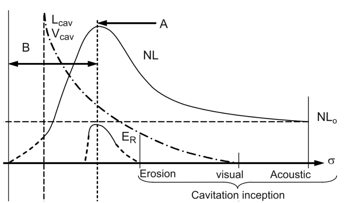
As can be seen from the figure above, when the cavitation coefficient or the inlet pressure is sufficiently high, the noise level is roughly constant and is due to the background noise of the pump running. Usually, this noise is generated by flow turbulence, unsteady blade forces, and mechanical noises. As the cavitation coefficient is reduced the noise level increases. This increase in the noise level is due to the cavitation bubbles being formed at the impeller inlet. The noise level keeps on increasing as the volume and the number of cavitation bubbles increases and reaches a maximum. The fall in the noise level left of region A is observed due to multiple reasons. Firstly, the potential energy of implosion resulting in the additional noise being generated depends both on the pressure differential and the bubble volume. The equation for cavitation bubble potential energy is as follows:
$$ E_pot = \frac{4}{3}\pi\left(R_o^3 – R_e^3\right)\left(p-p_v\right) \tag{16}$$
| Symbols | Meaning |
| \(R_o\) | bubble radius at when the cavity is formed |
| \(R_e\) | bubble radius at the end of the implosion |
| \(p_v\) | vapor pressure |
| \(p\) | fluid pressure surrounding the bubble |
As the inlet pressure reduces, the bubble radius increases but the pressure differential reduces. These counteracting phenomena result in a decrease in the potential energy and hence the noise. Moreover, as the cavitation bubble size and number increase, a certain amount of noise gets absorbed by the bubbles as gasses which are not as good a conductor of sound waves as the liquids, and this results in the noise level falling below the background noise. Moreover, it should be noted that in region A, there is a lag between the visual perception of the cavitation bubbles and the increase in the noise level above the background noise. This might be due to the development of microbubbles too small to detect visually.
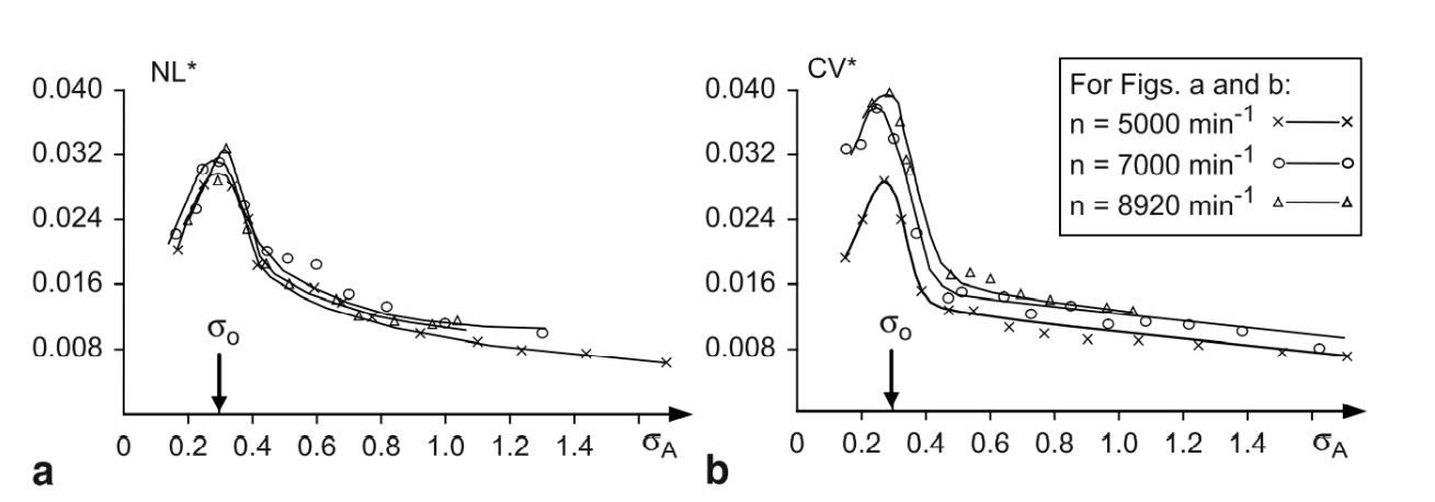
Figure 17 shows both the fluid-borne and solid-borne normalized noise levels for different rotation speeds. The solid-borne noise levels have been measured using an accelerometer outside the inlet casing. The solid-borne noise consists of background noise coming from the bearings, gearboxes, seals, etc. which are also dependent on the rotation speed that is why the curves do not fall on each other as they do in the case of fluid-borne noise.
Cavitation Prediction Using CFD
Due to both the extensive time and financial costs associated with physical prototyping and testing, engineers are increasingly relying upon the computational simulation of pumps.
Whereas physical benchmarking may take upwards of weeks, a CFD simulation in SimScale may only take minutes. This efficiency allows engineers to investigate exponentially more designs and push for higher-performing solutions within an allotted time frame. Furthermore, CFD results can readily and easily provide information such as where cavitation is occurring and at what flow rates/pressures it onsets. Tightening the loop between results and the design team enables iterative design where the strengths of previous designs can be carried forward and their deficiencies addressed.
Cavitation is typically modeled as an extension of the variable density Navier Stokes equations with an additional transport equation for the gaseous phase. This is coupled to the liquid phase via a set of source and sink terms based on local conditions such as pressure, turbulence, temperature, and more. A phase fraction term is introduced, representing the given content of a cell that is occupied by either gas or liquid.
How to Model Cavitation Using SimScale?
Technical Formulation
Simscale employs the full cavitation model proposed by Singal\(^9\) as a part of their turbomachinery solver. This formulation takes the three main drivers of cavitation into account and models each of them. These drivers are:
- formation and transport of vapor bubbles through the domain.
- local fluctuations in pressure and velocity due to turbulence.
- the expansion of entrained gas bubbles in the incoming flow.
The Rayleigh-Plesset equations for bubble dynamics are employed for modeling the rate of phase change. The empirical constants used in the equations have been calibrated with experiments over a wide range of applications and can be used as such for different problems. The effect of non-condensable gasses (i.e. dissolved or entrained air) is also included in the full cavitation model. The cavitation model in SimScale is well-validated for a variety of applications including submersible pumps, hydraulic turbines, control valves, and marine propellers.
Using the cavitation model in SimScale, it is possible to:
- determine NPSHr for a pump, by running parallel simulations on the cloud to generate the performance curve and assess when the performance falls below 3%.
- evaluate drop in efficiency due to cavitation and also predict pump performance in off-design conditions.
- predict cavitation damage by capturing bubble collapse and water hammer effects.
- predict noise and vibration due to cavitation by way of capturing the pressure pulses in the pump systems.
- capture the effect of non-condensable gasses entrained in the liquid.
The cavitation model in SimScale includes comprehensive physics as discussed above, while also implementing robust convergence logic to ensure successful simulations. Realistic material properties can be assigned and acute cavitation/aeration up to 15% can be handled.
How to Set Up a Cavitation Simulation in SimScale?
Cavitation capability is available within the Multi-purpose solver of SimScale. To learn how to prepare a centrifugal pump geometry and set it up for simulation in Multi-purpose, please refer to this tutorial.
Once you are familiar with setting up simulations in Multi-purpose, you can proceed to add the cavitation capability to the simulation tree. To simulate cavitation, a few more steps are required as described below:
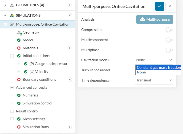
- Go to the main panel of the Multi-purpose solver, and for the Cavitation model option, select ‘Constant gas mass fraction’ from the dropdown menu. This is shown in Figure 18.
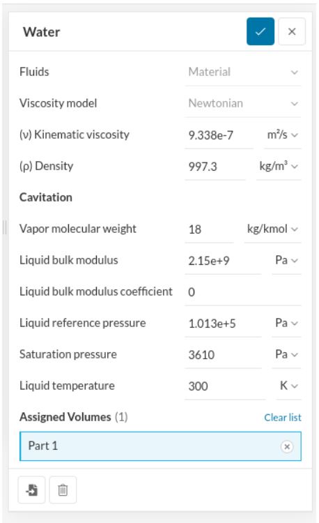
- Once cavitation is turned ON, you need to set up the material properties for the liquid that you would like to simulate. By default, water is set as the working fluid and its material properties are input at 300 K. It is possible to add any custom liquid in the ‘Materials’ panel as long as the user assigns correct values for Liquid bulk modulus, Saturation pressure, vapor’s molecular weight, etc. These properties are used to determine the onset of cavitation, for example, fluids with a higher saturation pressure will more readily vaporize and cause cavitation. The ‘Materials’ panel with water as the working fluid is shown in the figure below. This liquid should be assigned to the pump flow volume created in the CAD preparation step.
- The remaining setup of the simulation is exactly the same as without cavitation. The user should proceed to set up the correct boundary conditions, rotating zones, simulation, result controls, and finally the mesh parameters. When the simulation is run, the results will include the effects of cavitation, which is visualized in the form of vapor mass and volume fractions, as well as spikes in the fluid pressure at locations where bubble collapse happens.
How to Post-Process Cavitation Results in SimScale?
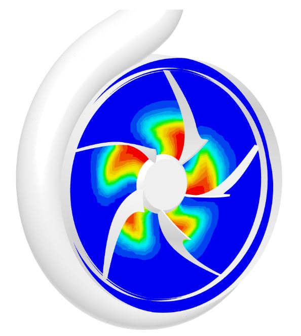
The effect of cavitation in a pump can be visualized in the form of vapor mass and volume fractions in the flow. If cavitation is included in the simulation, then the ‘Field Solution’ will include the total gas volume fraction for viewing. This represents the fraction of each cell that is filled by the gas phase, where 0 represents pure liquid (no vapor and, therefore, no cavitation) and 1 is pure gas.
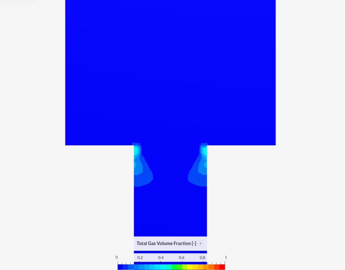
When the vapor mass fraction is greater than zero, it signifies the location of cavitation. For example, the image below shows that there is severe cavitation around the impeller blades of the centrifugal pump.
Simulate Cavitation yourself!
Do you also feel like simulating real life cavitation cases yourself and help in boosting your pump performance and life. All of All of this is possible by simply signing up as our Community or Professional SimScale user.
References
- “Cavitation and NPSH.” KSB, 22 February 2022, https://giw.ksb.com/blog/cavitation-and-npsh. Accessed 24 October 2022
- Visser, Frank. “Cavitation in Centrifugal and Axial-Flow Pumps.” 2022.
- Feng, Weimin. “Simulation of cavitation performance of an axial flow pump with inlet guide vanes.” Advances in Mechanical Engineering, vol. 8, no. 6, June 2, 2016, https://doi.org/10.1177/1687814016651583.
- “How to Avoid Pump Cavitation? 6 Main Steps.” Linquip, 22 August 2021, https://www.linquip.com/blog/what-is-pump-cavitation/. Accessed 24 October 2022.
- Nickerson, Philip. “Cavitation, the ‘pump disease’ – Responsible Seafood Advocate.” Global Seafood Alliance, 1 May 2007, https://www.globalseafood.org/advocate/cavitation-the-pump-disease/. Accessed 24 October 2022.
- “Phase Diagrams | Chemistry for Majors.” Lumen Learning, https://courses.lumenlearning.com/chemistryformajors/chapter/phase-diagrams-2/. Accessed 14 October 2022.
- Gülich, Johann Friedrich. Centrifugal Pumps. Springer Berlin Heidelberg, 2010. Accessed 7 October 2022.
- “File:PVT 3D diagram-en.svg.” Wikimedia Commons, https://commons.wikimedia.org/wiki/File:PVT_3D_diagram-en.svg. Accessed 13 October 2022.
- Singhal, A.K. et al. (2002) “Mathematical basis and validation of the full cavitation model,” Journal of Fluids Engineering, 124(3), pp. 617–624. Available at: https://doi.org/10.1115/1.1486223.
Last updated: November 26th, 2024
Did this article solve your issue?
How can we do better?
We appreciate and value your feedback.
What's Next
What is von Mises Stress?

