Documentation
The Transport equation describes how a scalar quantity is transported within a fluid and applies to many scalars, including passive scalars, temperature and even momentum by component. The general transport equation is as follows:
$$ \frac{\partial \phi}{\partial t} = – \mathbf{\nabla} \cdot \boldsymbol{u} \phi \hspace{2mm} + \mathbf{\nabla} \cdot \Gamma \mathbf{\nabla} \phi + S \tag{1}$$
Where:
\(\phi\) can be any scalar
\(\frac{\partial \phi}{\partial t}\) is the change of the scalar over time
\(\boldsymbol{u}\) is the velocity vector (\(u, v, w\))
\(\nabla\) is called nabla and represents the gradient of a scalar, but \(\mathbf{\nabla} \cdot\) represents the divergence of a scalar (we will break this down later also)
\(S\) is the source of a scalar
From the mathematical point of view, the transport equation is also called the convection-diffusion equation, which is a second-order linear PDE (partial differential equation). The convection-diffusion equation is the basis for the most common transportation models.
If this equation looks daunting to you, don’t worry, we will break it down in the coming paragraphs to show that it is surprisingly simple.
The transport equation can be seen as the generalization of the conservation equation:
$$ \frac{\partial \phi}{\partial t} = \mathbf{\nabla} \cdot J + S \tag{2}$$
Where:
\(J\) is the flux of a scalar
Let’s start by understanding the main components that get us from the continuity equation \(^2\) to the scalar transport equation \(^1\).
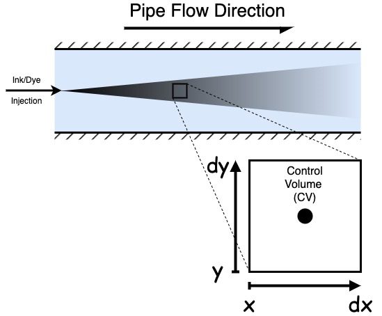
When discussing the mathematics behind the transport equation, we must be familiar with a few terms. Firstly, a control volume is a small, arbitrarily shaped fluid volume. When we consider the volumes in the context of CFD, they tend to be polyhedrally shaped volumes created when meshing. Many similarly shaped volumes exist.
We usually want to consider the volumes to be infinitesimally small, or their size tends towards zero. The smaller the volume, the more accurate our solutions become.
The principle of Scalar Transport Conservation states that the rate of change for a scalar quantity in any differential control volume is given by the flow and diffusion of the scalar into and out of the system, along with any generation or consumption inside the control volume.
In practice, the change of concentration of a certain quantity in the volume is the balance of the quantity flow across the boundary and the amount produced or removed inside the volume. From the mathematical point of view, we can express the balance using the equation\(^2\):
$$ \frac{\partial \phi}{\partial t} = \mathbf{\nabla} \cdot J + S \tag{2}$$
Flux \(J\) is the conservation of a transported quantity. Temperature, for instance, is not conserved, but heat flux is – and in our case we’re dealing with scalar flux. In fluids, we consider how the scalar moves with the fluid flow (Convection), but also, unrelated to the flow direction, how a scalar diffuses into the fluid (Diffusion).
Mathematically we can say:
$$ J = J_{convection} – J_{diffusion} \tag{3}$$
We will discuss later why diffusion has a negative convention, but maybe you can guess already.
We can write the terms as follows:
$$ J_{convection} = u \phi \tag{4}$$
$$ J_{diffusion} = \Gamma \mathbf{\nabla} \phi \tag{5}$$
where
\(\Gamma\) is the diffusion coefficient. The higher this value, the faster the diffusion
Convection:
Diffusion:
We can see that the flux term represents how a scalar moves spatially over time through convection and diffusion.
Source:
\(S\), the source term, represents the amount of the scalar quantity created or destroyed inside the control volume.
placing equation\(^4\) and equation\(^5\) into equation\(^3\), and equation\(^3\) into equation\(^2\) we get:
$$ \frac{\partial \phi}{\partial t} = \mathbf{\nabla} \cdot(- \boldsymbol{u} \phi + \Gamma \mathbf{\nabla} \phi) + S \tag{6}$$
Expanding the equation out gives the generalized form of the transport equation\(^1\):
$$ \underbrace{\frac{\partial \phi}{\partial t}}_{\substack{\text{unsteady} \\ \text{term}}} = \underbrace{- \mathbf{\nabla} \cdot \boldsymbol{u} \phi \vphantom{\frac{\partial \phi}{\partial t}}}_{\substack{\text{Convection} \\ \text{term}}} \hspace{2mm} + \underbrace{\mathbf{\nabla} \cdot \Gamma \mathbf{\nabla} \phi \vphantom{\frac{\partial \phi}{\partial t}}}_{\substack{\text{Diffusion} \\ \text{term}}} + \underbrace{S \vphantom{\frac{\partial \phi}{\partial t}}}_{\substack{\text{Source} \\ \text{term}}} \tag{1}$$
The transport equation forms the basis of most CFD codes, where from it the Navier Stokes Equations, Energy Equations, Species Equations and many other conservations can be derived.
Although each listed has a page in our SimWiki, let’s quickly go through some to show how they are derived from the transport equation.
During thermal simulations, the temperature field (which is scalar) will transport according to the convection-diffusion equation. In this specific case, the science community commonly uses the following notation.
$$ (\rho c_{p})\frac{\partial T}{\partial t} = – (\rho c_{p})\nabla\cdot (uT) \ + \nabla\cdot (k\nabla T) + \frac{Q_{\text{source}}}{V}$$
Where:
All terms in the equation have units \([mass^{1}][length^{-1}][time^{-3}]\) which is also known as the volumetric heat flux.
The source terms can also include terms for radiation or other contributions from complex interactions such as humidity.
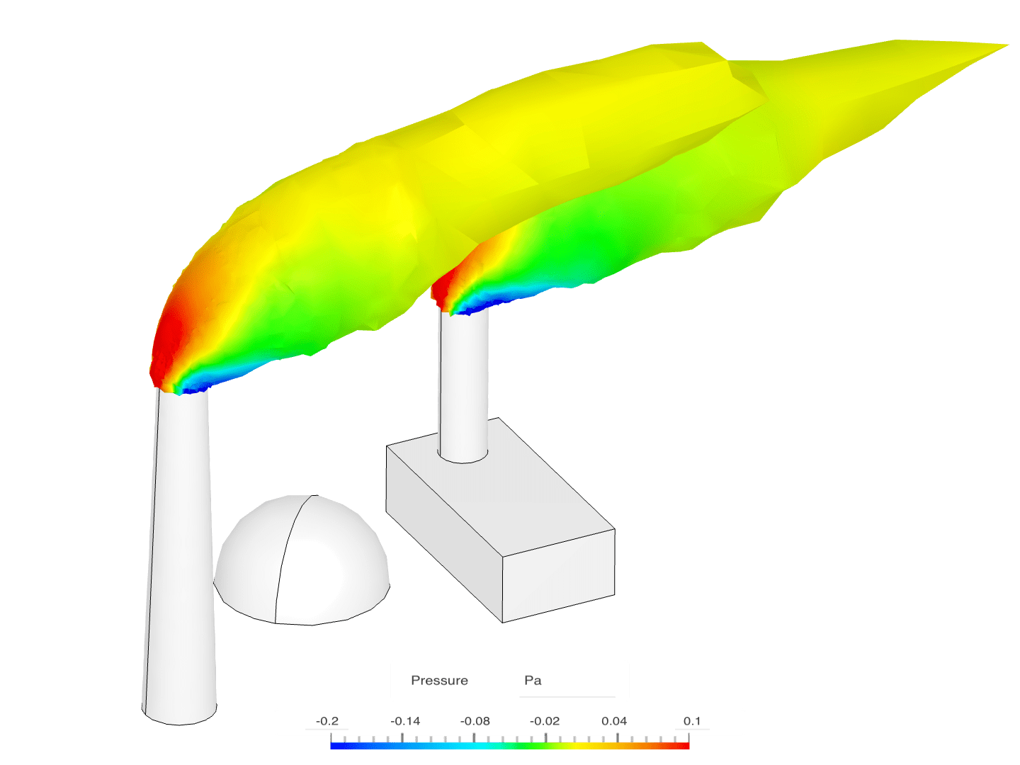
We consider many contaminants and pollutants to be Passive Scalars. A Passive Scalar is passive because it does not affect the flow field. An example of passive scalar use is tracking a contaminant from an industrial area, how it moves through the air and how it could affect the air quality of a residential area. This pollutant could be as simple as air with an undesirable smell. Passive scalars can also sometimes be referred to as passive species.
$$ \underbrace{\frac{\partial \phi}{\partial t}}_{\substack{\text{unsteady} \\ \text{term}}} = \underbrace{- \mathbf{\nabla} \cdot \boldsymbol{u} \phi \vphantom{\frac{\partial \phi}{\partial t}}}_{\substack{\text{Convection} \\ \text{term}}} \hspace{2mm} + \underbrace{\mathbf{\nabla} \cdot \Gamma \mathbf{\nabla} \phi \vphantom{\frac{\partial \phi}{\partial t}}}_{\substack{\text{Diffusion} \\ \text{term}}} + \underbrace{S \vphantom{\frac{\partial \phi}{\partial t}}}_{\substack{\text{Source} \\ \text{term}}} \tag{1}$$
A passive scalar uses the general transport equation as we defined in equation\(^1\), where:
The convective term describes how the pollutant moves with the velocity field.
The diffusion term describes how much the pollutant dispurses into the surrounding air.
The source term is used to inject the passive scalar into a volume. In the example, this could be a water processing plant or similar.
In SimScale, The diffusion coefficient \(\Gamma\) is defined in the model node within the simulation tree. The source term is defined in the Advance Concepts, within the simulation tree under Passive scalar sources as either a volumetric passive scalar source or a passive scalar source assigned to a volume or primitive.
Firstly, let’s consider what we are trying to achieve, a simple equation that describes how a scalar moves in the fluid. We do this with an eulerian frame of reference, i.e. the volume we consider is static, and the fluid moves in and out of that volume.
A good place to start is with a conservation equation, where we conserve some scalar concerning its concentration. Most of us know the conservation of mass, but if not, it is written as follows:
$$ \dot{m} = \rho.A. \boldsymbol{u} \tag{11}$$
If we express the mass flow rate as a function of volume, we can also get the equation:
$$ \frac{d \rho V}{d t} = \rho A \boldsymbol{u}$$ or more generically: $$ \frac{d \phi V}{d t} = \phi A \boldsymbol{u}\tag{12}$$
\(\phi\) can be any scalar concentration, with units \([\text{scalar unit}^{1}][length^{-3}]\). Scalar units could be anything appropriate to the problem.
If we re-arrange this and consider it for a very small volume:
$$ \frac{\partial \phi}{\partial t} = \frac{A \boldsymbol{u} \phi }{V} \tag{13}$$
\(\frac{\partial \phi}{\partial t}\) has units \([\text{scalar unit}^{1}][length^{-3}][time^{-1}] \)
We will do sanity checks at each major step in the following derivations to ensure the units for each term match these.
Let’s come back to that later and now consider the partial derivative, a change in scalar over time. The amount of scalar in a volume can change due to a few things, as we previously discussed, convection, diffusion and a source.
$$ \frac{\partial \phi}{\partial t} = – \frac{\partial \phi}{\partial t} \Bigr|_{convection} + \frac{\partial \phi}{\partial t} \Bigr|_{diffusion} + \frac{\partial \phi}{\partial t} \Bigr|_{source}\tag{14}$$
The reason we write the above step is to make us less prone to error. As a student, much time was wasted when equations got too long for my page, and things were missed or squashed unreadably at the end.
The convection term is the easiest of the two fluxes. Let’s return to the equation:
$$ \frac{\partial \phi V}{\partial t}\Bigr|_{convection} = \boldsymbol{u} \phi A \tag{15}$$
In the following steps, we introduce a symbol \(J\) that represents flux. Flux is a common term in fluid dynamics and represents how much scalar flows through an arbitrary boundary. It has units of \([\text{scalar unit}^{1}][length^{-2}][time^{-1}]\).
A convective flux can be written as follows:
$$ J = \boldsymbol{u} \phi \tag{16}$$
And substituting flux into equation\(^{15}\), we can separate the flux for simplicity. This is less important for the convection term but is very helpful later for the diffusion term so that we will be consistent.
$$ \frac{\partial \phi V}{\partial t}\Bigr|_{convection} = JA \tag{17}$$
To take this further, the total flux will be split into a few components, into flux in minus flux out:
$$ \frac{\partial \rho \phi V}{\partial t}\Bigr|_{convection} = J_{out}A – J_{in}A \tag{18}$$
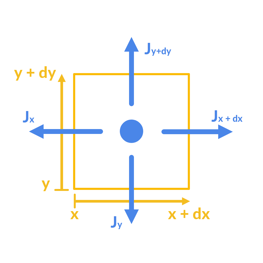
But also, we can split these components into x and y components.
We are deriving the transport equation in two dimensions here, but it is just as applicable to 1D or 3D problems. We will generalise it to n dimensions at the end. As a 2D derivation, the volume is two-dimensional, and the area is one-dimensional.
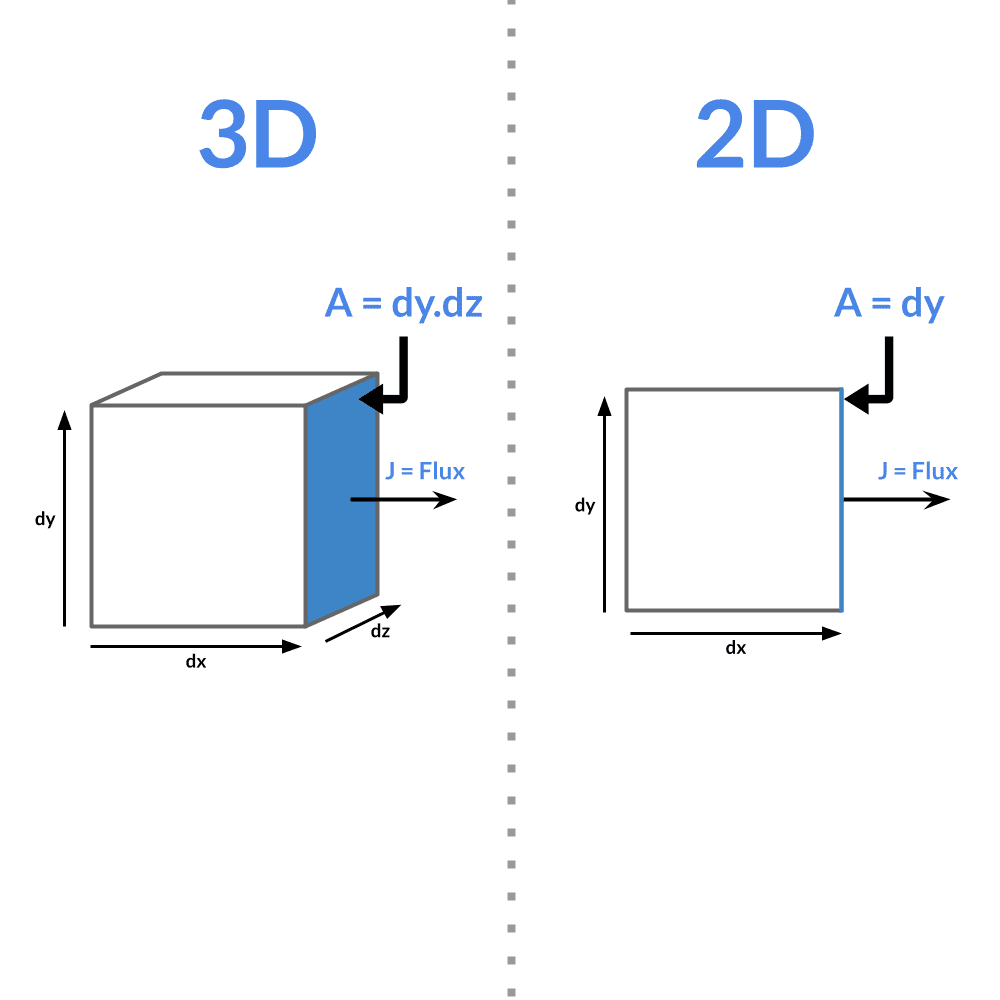
So in our convention, in 2D, the area of the low x boundary is dy so that we can write flux in by area and flux by area out as:
$$ J_{in}A = J\Bigr|_{x}.dy + J\Bigr|_{y}.dx\tag{19} $$
$$ J_{out}A = J\Bigr|_{x+dx}.dy + J\Bigr|_{y+dy}.dx\tag{20} $$
We do this at this stage because, like the flux is per boundary, the area is per boundary.
Substituting equation\(^{16}\)back into J:
$$ J_{in}A = \phi u\Bigr|_{x}.dy + \phi v\Bigr|_{y}.dx\tag{21} $$
$$ J_{out}A = \phi u\Bigr|_{x+dx}.dy + \phi v\Bigr|_{y+dy}.dx\tag{22} $$
Notice how the velocity component changes with direction. We can express the velocity vector as a bold symbol, where it represents all three components in a 3D problem:
$$ \boldsymbol{u} = (u, v, w) $$
substituting equations\(^{21,22}\) into equation\(^{18}\) we get:
$$ \frac{\partial \phi V}{\partial t}\Bigr|_{convection} = \phi u \Bigr|_{x+dx}.dy – \phi u \Bigr|_{x}.dy + \phi v \Bigr|_{y+dy}.dx – \phi v\Bigr|_{y}.dx \tag{23}$$
We also know volume \(V = dx.dy\) in two dimensions. dividing equation\(^{23}\) by \(dx.dy\) we get:
$$ \frac{\partial \phi}{\partial t}\Bigr|_{convection} = \frac{\phi u\Bigr|_{x+dx}.dy – \phi u\Bigr|_{x}.dy}{dx.dy} + \frac{ \phi v \Bigr|_{y+dy}.dx – \phi v \Bigr|_{y}.dx}{dx.dy} \tag{24}$$
Simplifying to become:
$$ \frac{\partial \phi}{\partial t}\Bigr|_{convection} = \frac{\rho u \Bigr|_{x+dx} – \phi u \Bigr|_{x}}{dx} + \frac{\phi v \Bigr|_{y+dy} – \phi v \Bigr|_{y}}{dy} \tag{25}$$
Since this is a partial derivative, we can rewrite it as:
$$ \frac{\partial \phi}{\partial t}\Bigr|_{convection} = \frac{\partial \phi u}{\partial x} + \frac{\partial \phi v}{\partial y} \tag{26}$$
Lets us again take a pause and talk about Nabla \(\nabla\) as just a way of simplifying some of these terms and making them more general to n-dimensional problems. \(\nabla\) can sometimes be called gradient. However, it’s not strictly that. For a scalar, we can write:
$$ \nabla \phi = (\frac{\partial \phi}{\partial x}, \frac{\partial \phi}{\partial y}, \frac{\partial \phi}{\partial z}) \tag{27}$$
However, for a vector, like \(\boldsymbol{u}\):
$$ \nabla \boldsymbol{u} = (\frac{\partial u}{\partial x}, \frac{\partial v}{\partial y}, \frac{\partial w}{\partial z}) \tag{28}$$
Another thing to consider is \(\nabla \cdot\) or called divergence:
$$ \nabla \cdot \boldsymbol{u} = \frac{\partial u}{\partial x} + \frac{\partial v}{\partial y} + \frac{\partial w}{\partial z} \tag{29}$$
This takes us to our final simplification step. notice how we have something almost identical to \(\nabla \cdot\) in equation\(^{25}\) lets substitute in equation\(^{29}\) for \(\nabla \cdot \phi \boldsymbol{u}\):
$$ \boxed{\frac{\partial \phi}{\partial t}\Bigr|_{convection} = \nabla \cdot \boldsymbol{u} \phi }\tag{30}$$
Now we really should check to make sure our derivation of the convection term matches the expected units. Earlier, it was mentioned that the change in scalar concentration had the units of \([\text{scalar unit}^{1}][length^{-3}][time^{-1}]\) so if the scalar unit was kg, and we were in metric units, it would be something like \(\frac{kg}{m^{3}s}\).
Now if we take \(\nabla \cdot \boldsymbol{u} \phi\) and express it in 1D, we get \(\frac{\partial \boldsymbol{u} \phi}{\partial x}\). Writing out the units, assuming scalar units are kg’s and we are using the metric unit system:
\(\phi = \frac{kg}{m^{3}}\)
\(u = \frac{m}{s}\)
\(\frac{\partial}{\partial x} = \frac{1}{m}\)
Simplifying this and making it general to a unit system and using the scalar units, we can write this as \([\text{scalar unit}^{1}][length^{-3}][time^{-1}]\), which matches our expectation, and proves we made no mistakes so far. This is a good practice and will ultimately save you time in the long run.
In the convection term, we knew that a scalar \(\phi\) was transported with the flow field \(\boldsymbol{u}\) and formed the basis for the flux \(J= \boldsymbol{u} \phi \) based upon the scalar conservation equation. Similarly, for the diffusion term, we need to define \(J\). In diffusion, the difference in scalar concentration plays a strong role, where we intuitively know in one dimension:
$$ J \propto \frac{d \phi}{ d x} \tag{31}$$
Now, if we put a constant in to make an equation, you might notice it looks a lot like Flick’s First Law, so instead of putting any constant in, let’s put the diffusion coefficient in. Also, since a diffusion coefficient is a positive number, but a scalar will move from high concentration to low (a negative gradient), we must also introduce a negative constant.
$$ J = – \Gamma \frac{d \phi}{ d x} \tag{32}$$
If we wanted to look at this in multiple directions, we could say for two dimensions:
$$ \boldsymbol{J} = (- \Gamma \frac{d \phi}{ d x}, – \Gamma \frac{d \phi}{ d y}) = -\Gamma \nabla \phi \tag{33}$$
Using the same convention as before, equation\(^{18}\), but this time we consider for diffusion:
$$ \frac{\partial \phi V}{\partial t}\Bigr|_{diffusion} = J_{out}A \; – \; J_{in}A \tag{34} $$
As before in convection, we use the same convention to define the diffusion in and out:
$$ J_{in}A = J\Bigr|_{x}.dy + J\Bigr|_{y}.dx\tag{35} $$
$$ J_{out}A = J\Bigr|_{x+dx}.dy + \Bigr|_{y+dy}.dx\tag{36} $$
However, at this stage, we have a dilemma. If we substitute in J, we would have difficulty simplifying the derivatives from equation\(^{32}\). Luckily, we have some assistance available from the Taylor series expansion. Taylor series expansion to the first order is as follows:
\(f(x) = f(a) + f'(a).(x-a)\) or specifically for our problem, \(f(x+dx) = f(x) – f'(x).dx\)
And we can substitute that into equation\(^{36}\):
$$ J_{out}A = J\Bigr|_{x}\partial y \; – \; \frac{\partial J}{\partial x}.\Bigr|_{x} \partial x \partial y + J\Bigr|_{y} \partial x \; – \; \frac{\partial J}{\partial y}.\Bigr|_{y} \partial y \partial x\tag{37}$$
Substituting equations\(^{35,37}\) into equation\(^{34}\) we would get:
$$ \frac{\partial \phi V}{\partial t}\Bigr|_{diffusion} = J\Bigr|_{x} \partial y \; – \; \frac{\partial J}{\partial x}.\Bigr|_{x} \partial x \partial y + J\Bigr|_{y} \partial x \; – \; \frac{\partial J}{\partial y}.\Bigr|_{y} \partial y \partial x – \left ( J\Bigr|_{x} \partial y + J\Bigr|_{y} \partial x \right ) \tag{38} $$
Which simplifies into:
$$ \frac{\partial \phi V}{\partial t}\Bigr|_{diffusion} = – \left ( \partial J\Bigr|_{x} \partial y + \partial J\Bigr|_{y} \partial x \right ) \tag{39} $$
And as before, volume \(V=\partial x \partial y\), dividing equation\(^{39}\) by \(V\) gives:
$$ \frac{\partial \phi}{\partial t}\Bigr|_{diffusion} = – \left ( \frac{\partial J\Bigr|_{x}}{\partial x} + \frac{\partial J\Bigr|_{y}}{\partial y} \right ) \tag{40} $$
Now, recognising that \(\nabla \cdot \boldsymbol{J}\) because of its definition in equation\(^{29}\) we can rewrite this as:
$$ \frac{\partial \phi}{\partial t}\Bigr|_{diffusion} = – \nabla \cdot \boldsymbol{J} \tag{41}$$
and substituting in equation\(^{33}\) to equation\(^{41}\) we obtain the final diffusion term:
$$ \boxed{\frac{\partial \phi}{\partial t}\Bigr|_{diffusion} = \ – \nabla \cdot (- \Gamma \nabla ) \phi = \nabla \cdot \Gamma \nabla \phi }\tag{42}$$
Again, we should double-check the units. The diffusion term in 1D looks like what most would recognise as Flick’s Second Law \( – \Gamma \frac{\partial^{2} \phi}{\partial x^{2}}\).
\(\Gamma\) has units of \([length^{2}][time^{-1}]\)
\(\frac{\partial^{2}}{\partial x^{2}}\) has the units of \([length^{-2}]\)
\(\phi\) has units of \([\text{scalar unit}^{1}][length^{-3}]\)
Adding all the units we have \([\text{scalar unit}^{1 mm}][length^{-3}][time^{-1}]\) which is what we expect.
The source term is simple in contrast to the convection and diffusion terms. Since this is a direct addition to the transport equation, adding the concentration over time to the volume, it is expressed as:
$$ \boxed{\frac{\partial \phi}{\partial t}\Bigr|_{source} = S} \tag{43}$$
We can now see why it was easier to split the transport equation into three terms and substitute it at the end. If your following along to this with a pen and paper, you might be relieved. The last step takes equations 30, 42, 43, and substitutes them into equation14 to arrive at equation 1:
$$ \underbrace{\frac{\partial \phi}{\partial t}}_{\substack{\text{unsteady} \\ \text{term}}} = \underbrace{- \mathbf{\nabla} \cdot \boldsymbol{u} \phi \vphantom{\frac{\partial \phi}{\partial t}}}_{\substack{\text{Convection} \\ \text{term}}} \hspace{2mm} + \underbrace{\mathbf{\nabla} \cdot \Gamma \mathbf{\nabla} \phi \vphantom{\frac{\partial \phi}{\partial t}}}_{\substack{\text{Diffusion} \\ \text{term}}} + \underbrace{S \vphantom{\frac{\partial \phi}{\partial t}}}_{\substack{\text{Source} \\ \text{term}}} \tag{1}$$
Last updated: July 14th, 2025
We appreciate and value your feedback.
What's Next
What Are the Navier-Stokes Equations?Sign up for SimScale
and start simulating now


