Elasto-plastic Materials

A purely plastic material model describes the material behavior after the onset of plasticity. At this point, the solid materials will undergo irreversible deformation when subjected to loading. For example, a solid metal being shaped by bending or pounding.

In reality, most of the materials have an elastic and a plastic region separated by a yield point, after which the stress-strain curve becomes nonlinear. A typical stress-strain curve for steel is shown below:

Stress-strain curve for a ductile material. — Figure 1: Engineering stress-strain curve for a ductile material. (Source: Nicoguaro / CC BY)

That is why SimScale allows you to model such materials as elasto-plastic materials. The Elasto-plastic material model has a wide variety of applications, thus it is particularly useful for predicting the behavior of materials under extreme conditions, such as impact loading, high pressures, and high temperatures.

There are also applications where some plastic deformation is allowed in the design. In such cases, first run a simulation using a linear elastic behavior for the materials. If the stresses are greater than the yield strength, then an additional analysis is done with a plastic material behavior.

Important

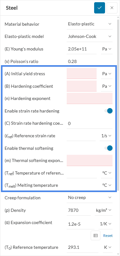
An elasto-plastic material behavior can only be defined for the following analysis types:

– Nonlinear static analysis;
– Dynamic analysis;
– Nonlinear thermomechanical analysis.

Elasto-plastic Model

A material which undergoes an elasto-plastic regime can be modeled as Bilinear, Multilinear or via Johnson-Cook parameters.

Multilinear Model

Modeling the material as multilinear means establishing its properties as being the same as the stress-strain curve obtained from a tensile test. In this model, the strain hardening curve is plotted by some linear lines tangent to the nonlinear behavior. Therefore, in multilinear modeling the material behaves as closely as possible to reality.

Bilinear Model

The bilinear hardening model is similar to the multilinear model, but it does not take into account the entire behavioral history of the material. This model is also described by the stress-strain curve, where the coefficients needed for material characterization are the Young modulus, and the plastic phase modulus, where the second one cannot be less than zero, neither greater than the Young modulus. When the plastic phase modulus comprises 99% of the Young modulus, the bilinear model simulates a linear elastic analysis. If the plastic phase modulus is 1% and/or 0, the bilinear model simulates the behavior of perfect plasticity.

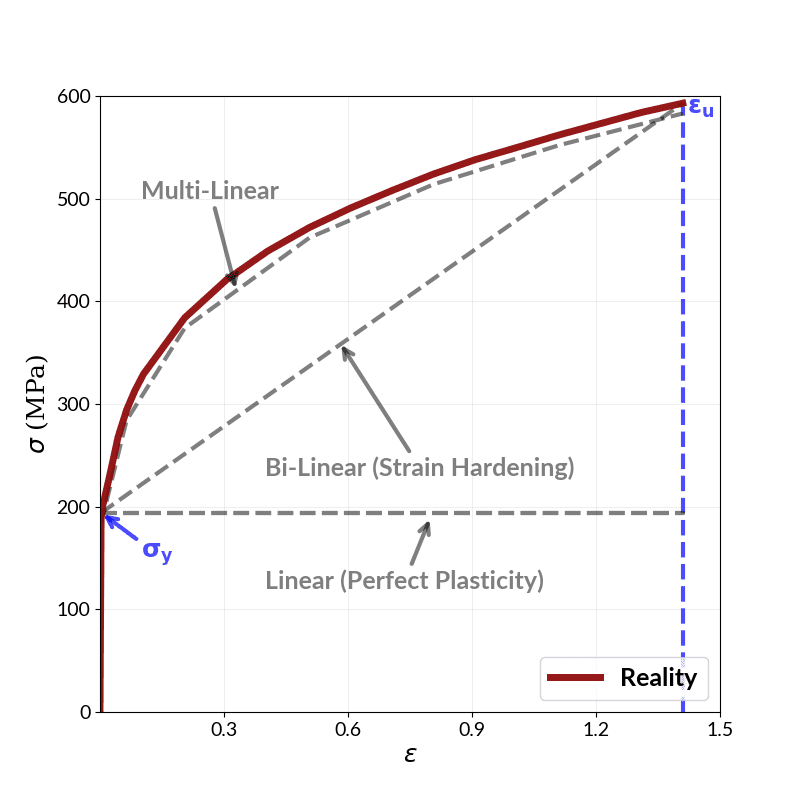
Stress-strain curve comparison, multilinear, bilinear and perfect plasticity. — Figure 2: Visual comparison between different elasto-plastic models (multilinear, bilinear, and perfect plasticity) and the real material curve.

As shown in Figure 2, the bilinear elasto-plastic model can be assumed to be sufficient to predict the behavior of materials when there is no complexity in terms of geometries and loadings in the simulation.

Quick Tip

The bilinear material model provides a handy modeling tool with a good approach, once it is simple and quick. However, if you need to be more accurate, or if you have a complex model, prefer to use multilinear.

Notwithstanding, once you have chosen the bilinear elasto-plastic model, SimScale also provides perfect plasticity as an option for the hardening model. In general, perfect plasticity is a simplification of the actual material behavior, and it is only applicable under 2 situations:

The material does not strain harden;
The material is not subjected to cyclic loads.

Johnson-Cook Model

Another apporach would be to use the Johnson-Cook model [2], which is a widely used material model for capturing the stress – strain relationship in metallic materials, particularly in scenarios characterized by substantial deformation, high strain rates, and elevated temperatures. Renowned for its simplicity and ease of material constant estimation, this model is frequently used to predict the flow behavior of various materials. The flow stress model is expressed as:

$$\displaystyle \sigma = (\mathrm{A} + \mathrm{B}\mathrm{\varepsilon_{pl}^n}) \left ( 1 + \mathrm{C} \log(\mathrm{\dot{\bar{\varepsilon}}})\right )\left ( 1 – \mathrm{\bar{T}^m} \right) \tag{1}$$

where, $\sigma$ represents the equivalent stress, while $\varepsilon_{\mathrm{pl}}$ signifies the equivalent plastic strain. The model relies on several material constants, each playing a distinct role in shaping the material’s response:

$\mathrm{A}$: yield stress of the material under reference conditions.

$\mathrm{B}$: strain hardening constant under reference conditions.
$\mathrm{n}$: strain hardening exponent under reference conditions.
$\mathrm{C}$: strengthening coefficient of strain rate.
$\mathrm{m}$: thermal softening coefficient.

Breaking down Equation (1), the three components from left to right account for the strain hardening effect, the strain rate strengthening effect, and the temperature effect. These components collectively influence the flow stress values. In the context of the flow stress model, additional dimensionless parameters come into play:$$\dot{\bar{\varepsilon}} = \frac{\dot{\varepsilon}}{\dot{\varepsilon}_{\mathrm{ref}}}, \; \bar{\mathrm{T}} = \frac{\mathrm{T} – \mathrm{T_{ref}}}{\mathrm{T_{melt}} – \mathrm{T_{ref}}}$$

$\dot{\varepsilon}$: dimensionless strain rate.
$\bar{\mathrm{T}}$: homologous temperature
$\mathrm{T_{melt}}$: material’s melting temperature.
$\mathrm{T}$: deformation temperature.
$\dot{\varepsilon}_{ref}$: reference strain rate, usually representing a quasi-static process.
$\mathrm{T_{ref}}$: reference deformation temperature, usually represented by the room temperature.

These components interact dynamically within the Johnson-Cook model, allowing to analyze and predict material behavior across a spectrum of complex conditions, including those involving significant deformation, high strain rates, and elevated temperatures.

Defining Elasto-Plastic Materials in SimScale

Engineering Stress-Strain vs. True Stress-Strain

While most material parameters in practice are provided as engineering stress-strain, SimScale requires true stress-strain material properties to accurately cope with the thinning of the material.

Engineering vs. True Stress Strain

For ductile materials, thinning of the probe during material test can occur. Since stress is calculated as $$ Stress=\frac{Force}{Cross \ section} = \frac{N}{m^2} \tag{1}$$
two material parameters can be obtained — Engineering stress, which uses the initial cross-section as a reference, and true stress, which uses the true cross-section of the material.

To convert the engineering stress-strain data to true stress-strain the following formulas shall be used.

$$ \sigma_t = \sigma_e*(1+\varepsilon_e) \tag{2} $$

$$ \varepsilon_t = ln(1+\varepsilon_e) \tag{3} $$

Where,

$ \sigma_t $ = true stress
$ \varepsilon_t $ = true strain
$ \sigma_e $ = engineering stress
$ \varepsilon_e $ = engineering strain
$ln$ = natural log

In addition sometimes instead of engineering stress-strain curve the material data is provided as true stress-plastic strain curve. In such a case, this also needs to be converted to true stress – true strain. The following equation 4 can be used to convert this data.

$$ \varepsilon_t = \varepsilon_p + \frac{\sigma_t}{E} \tag{4} $$

Where,

$ \varepsilon_p $ = plastic strain
$ E $ = Young’s Modulus

Setup in SimScale

To define an elasto-plastic material, follow the steps given below:

Navigate to the Materials tab, in the simulation tree. Change the Material behavior to Elasto-plastic.
After choosing material behavior, the user needs to choose the elasto-plastic model (multilinear, bilinear or Johnson-Cook). Once the user selects multilinear, it is needed to input data for the stress-strain curve, as shown in the first column of Figure 3. Please note that the stress-strain curve should be true stress versus true strain.
If the user sets the material as bilinear, it is just necessary to decide between perfect plasticity or strain hardening model, considering the previous explanation in this article.
For the Johnson-Cook model, the user needs to define the parameters of interest – namely $\mathrm{A}$, $\mathrm{B}$ and $\mathrm{n}$ (also $\mathrm{C}$ and $\dot{\varepsilon}_{\mathrm{ref}}$ in case of strain rate hardening and $\mathrm{m}$, $\mathrm{T_ref}$ and $\mathrm{T_melt}$ in case of thermal softening) – as described in the previous section.

Bilinear and Multilinear

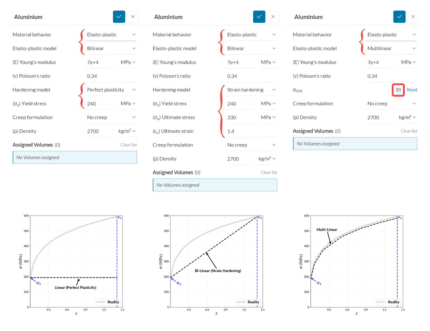
Figure 3 shows some examples of an elasto-plastic material – aluminum, for each case that the user is modeling as Bilinear with perfect plasticity, Bilinear with Strain hardening and Multilinear:

SimScale setup according to the stress-strain curve behavior. — Figure 3: Example of a SimScale material setup for aluminum as multilinear elasto-plastic model, perfect plasticity, and bilinear strain hardening, respectively.

with the obtained values shown in the Figure below.

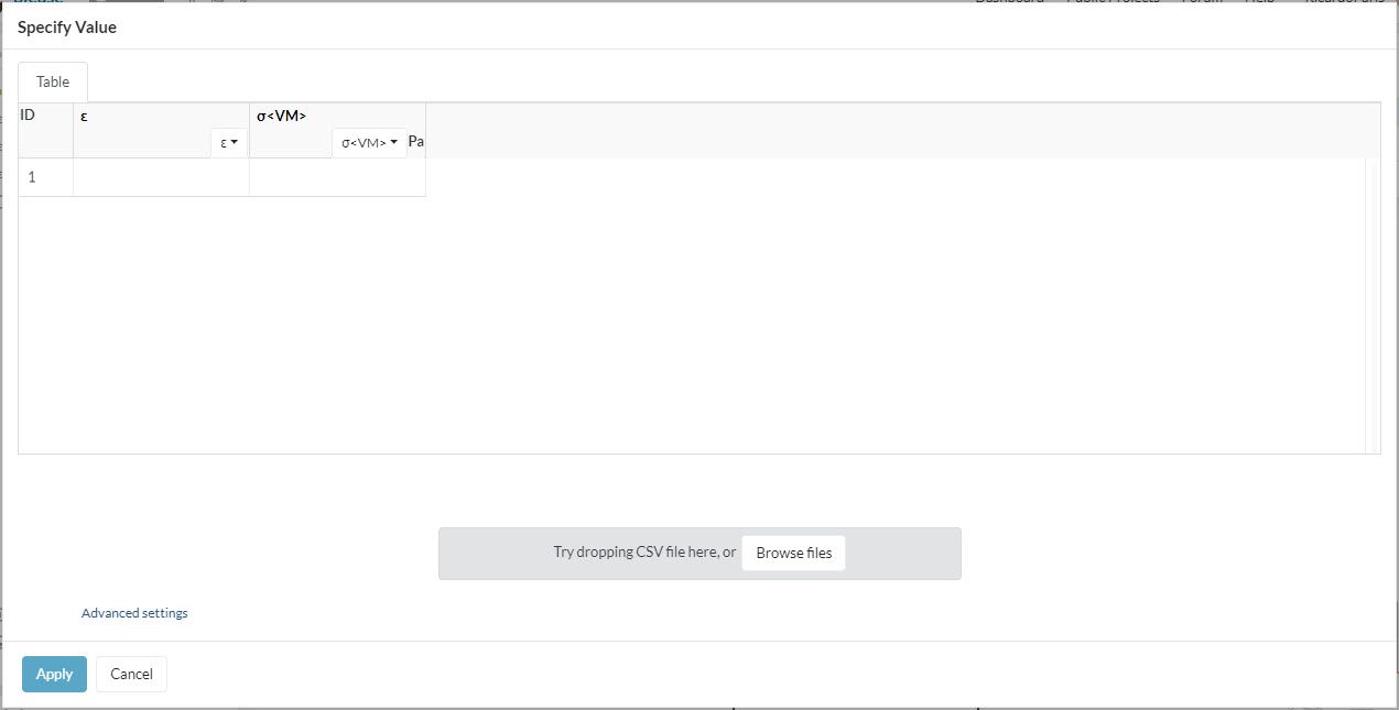
sample stress-strain curve for aluminum — Figure 4: Sample stress-strain curve for aluminum.

Once the user has chosen a multilinear model, a series of data points over the stress-strain curve and its coordinates are defined. These points can be manually input. Alternatively, it’s also possible to create a comma-separated .csv file in any text editor, containing the point coordinates in this format (no spaces after the comma): strain, stress. This .csv file can be uploaded to SimScale.

input stress strain curve in simscale — Figure 5: Table input for the stress-strain curve

Important

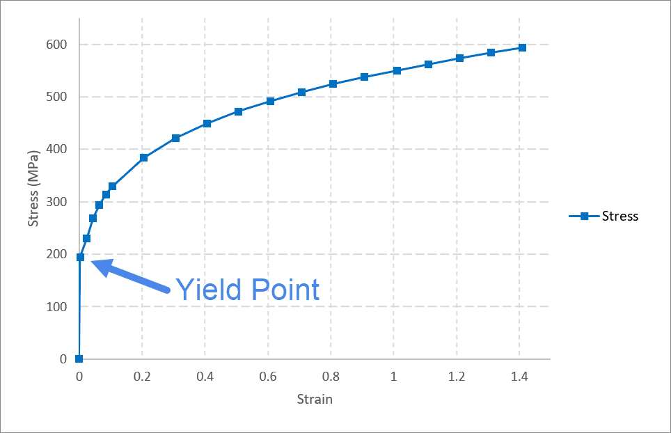
When using the multilinear model, the first point of the series is taken as the yield point by the solver. Using Figure 4 as reference, this would be the structure of the .csv file:

stress strain input aluminium set up — Figure 6: Stress-strain curve for aluminium.

To capture the stress-strain curve appropriately, make sure to add enough data points. Between two points, the values are linearly interpolated.

After saving the stress-strain curve, adjust Young’s modulus according to the stress-strain data. Young’s modulus is given by dividing the stress and strain values at the yield point:

$$E = \displaystyle \frac {\sigma_{yield}}{\varepsilon_{yield}} \tag {5}$$

After inputting the values from our example in equation (5), we have:

$$ \displaystyle E = \frac {1.94e8}{2.75e(-3)} = 7.05e10 \ Pa \tag {6}$$

A wrongly calculated value for Young’s modulus may lead to a diverged solution.

Note

This model is not a suitable choice for brittle materials such as ceramics and concrete. It is only applicable for ductile and isotropic materials, such as aluminum and steel.

Johnson-Cook

The Johnson-Cook model differs significantly from standard elasto-plastic models, as it accounts for both thermal softening and strain rate hardening. As a result, the stress-strain response is not unique; instead, it varies depending on the strain rate and operating temperature.

To set up Johnson-Cook parameters in SimScale, users typically need multiple stress-strain curves for a single material under varying conditions. Curve-fitting algorithms are then used to extract the model parameters from these curves. For commonly used materials, it is often possible to obtain the Johnson-Cook coefficients directly from existing literature.

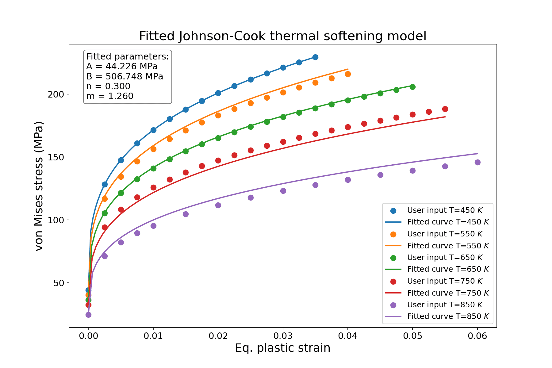
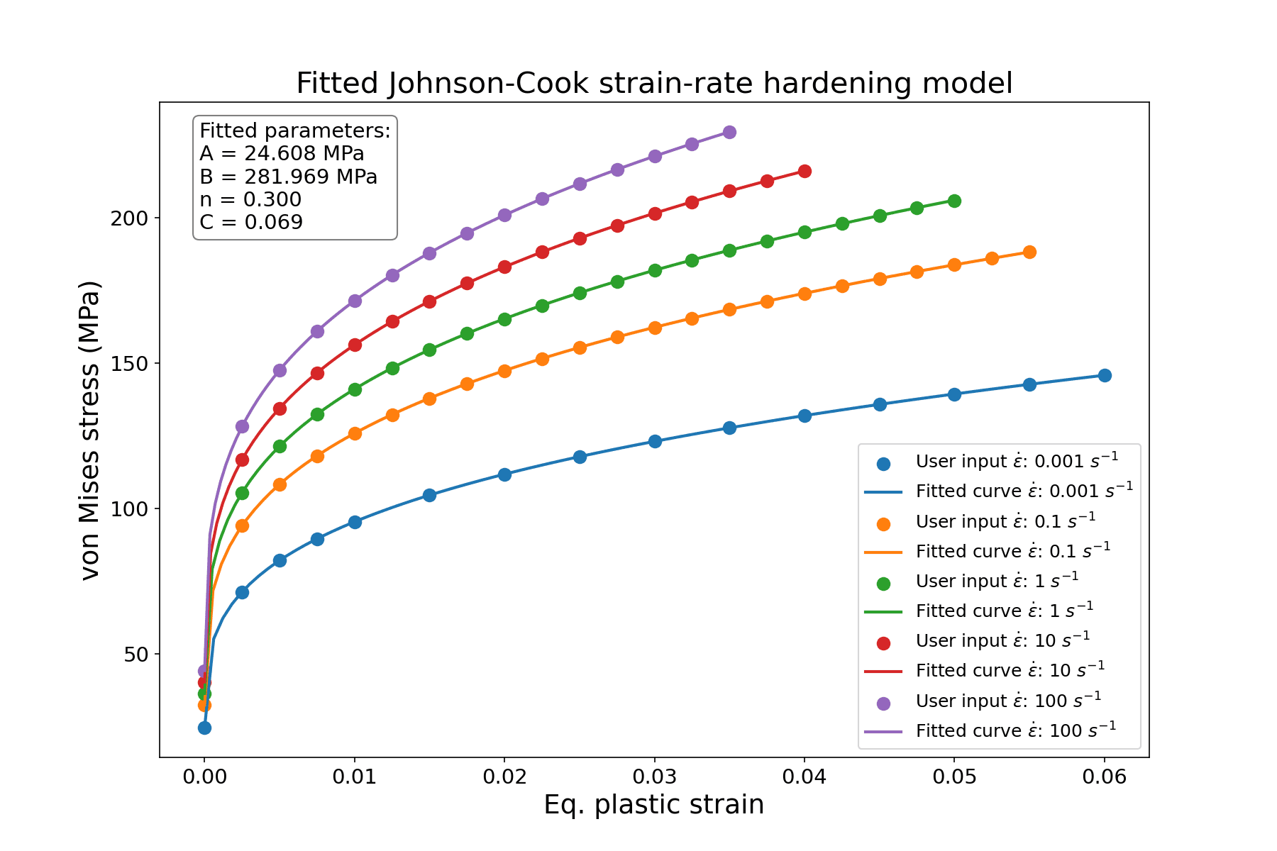
multiple thermal softening curves johnson cook model — (a) Thermal softening

multiple strain rate harnening curves for Johnson Cook model — (a) Thermal softening

Fig 7: Plotted curves examples for different Temperatures (a) and Strain-rates (b)

To fully utilize all features of the Johnson-Cook model, the user must set up a nonlinear Thermomechanical simulation, which incorporates both thermal softening and strain rate hardening. Strain rate hardening can also be applied in dynamic simulations and nonlinear static analyses.

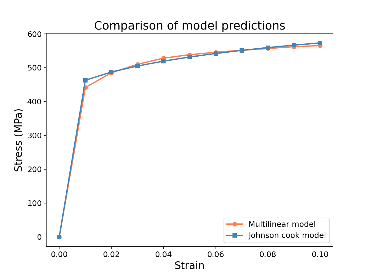
Fig 8: Parameter setting for the Johnson-Cook model using the Thermomechanical solver

When using the power-law approach (C and m coefficients set to zero) with a single stress-strain curve, the resulting behavior is generally comparable to that of the Multilinear material model, as shown in the Figure below.

model predictions multilinear vs johnson cook — Fig 9: Comparison between Johnson-Cook and Multilinear models

Projects

References

Last updated: June 17th, 2025

Did this article solve your issue?

How can we do better?

We appreciate and value your feedback.