Fill out the form to download

Required field
Required field
Not a valid email address
Required field
Required field
  • Set up your own cloud-native simulation in minutes.

  • Surface Load

    In the Surface Load boundary condition, a distributed load per unit area is applied on a face (or set of faces). It is useful to model the loads applied through the surface in contact with fluids or other solids, where the direction of application of the load is known beforehand, in terms of the global coordinate system components.
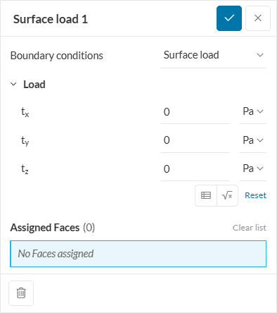
    surface load boundary condition parameters
    Figure 1: Surface load boundary condition panel. Enter the value in each direction with appropriate units and pick faces to assign.

    The parameters of the boundary condition are:

    1. Load: The components of the applied load, expressed in the global coordinate system directions of the model \( (t_x, t_y, t_z) \).
    2. Assignment: Set of faces where the surface load will be applied.

    Supported Analysis Types

    The following analysis types support the usage of this boundary condition:

    Resultant Force Magnitude and Direction

    The traction vector is defined by the components of the load:

    $$ \vec{t} = (t_x, t_y, t_z) $$

    Each component has units of force (\(N\), \(lb.\), etc) per unit of surface area (\(m^2\), \(sq. in.\), etc). Thus the traction has the units of pressure (\(Pa\), \(psi\), etc). The total applied force vector over the assignment set depends on the surface area of the assigned faces:

    $$ \vec{F} = \int \vec{t} dA $$

    Variable Load

    Variable surface load values can be specified with the use of the formula or table inputs. The allowed functions are:
    • Time-dependent: The pressure varies with respect to time (variable t) in a nonlinear static or dynamic simulation. This is useful, for instance, to ramp up the load from zero in nonlinear simulations, where a sudden application of load leads to numerical divergence, or for naturally time-varying loads in dynamic simulations.
    • Coordinate-dependent: The surface load varies with respect to the position in space (variables X, Y, Z).

    Maximum Number of Table Parameters

    Due to numerical difficulties, the underlying structural solver (Code_Aster) only supports table function definitions of one or two variables. If you need to define a function of the three spatial coordinates (X, Y, Z), or even combine it with time, you must create an analytical formula for it.

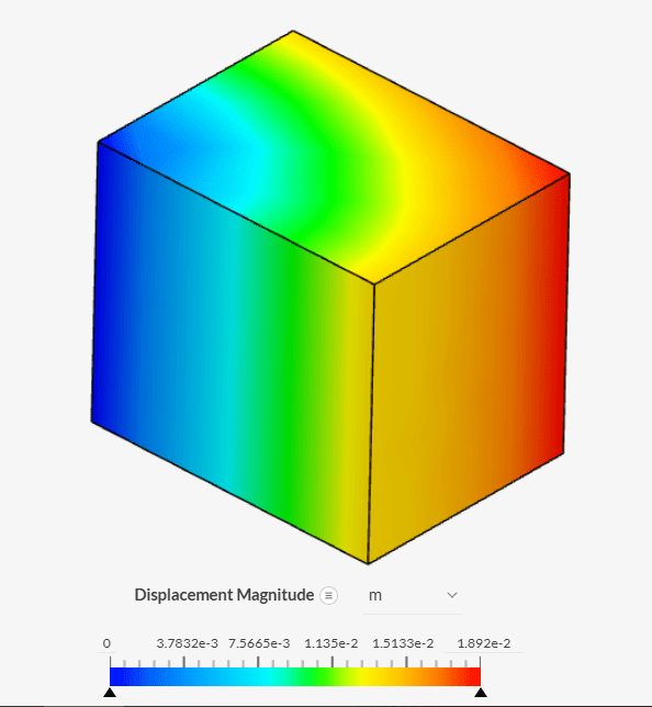
    surface load application example
    Figure 2: Deformation contour plot of a cube under triaxial surface load (see validation case below).

    Last updated: September 26th, 2022

    Contents