Validation Case: 3D Triaxial Load Secondary Creep (NAFEMS Test 6(a))
This triaxial load secondary creep validation case belongs to solid mechanics. This test case aims to validate the following parameters:
- Creep material behavior
- Standard and reduced integration elements
- Automatic time stepping
The simulation results of SimScale were compared to the analytical results derived from [NAFEMS_R27]\(^1\).
Geometry
The geometry consists of a cube with an edge length \(l\) = 0.1 \(m\).
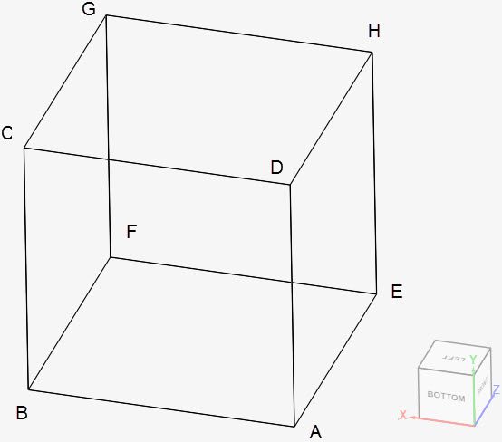
The coordinates for the points in the cube are as tabulated below:
| A | B | C | D | E | F | G | H | |
| x | 0 | 0.1 | 0.1 | 0 | 0 | 0.1 | 0.1 | 0 |
| y | 0 | 0 | 0.1 | 0.1 | 0 | 0 | 0.1 | 0.1 |
| z | 0 | 0 | 0 | 0 | 0.1 | 0.1 | 0.1 | 0.1 |
Analysis Type and Mesh
Tool Type: Code Aster
Analysis Type: Nonlinear static
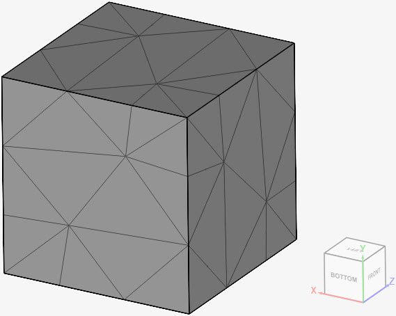
Mesh and Element Types: For this validation case, a single second-order tetrahedral mesh was created in SimScale with the standard algorithm.
The secondary creep formulation and element technology vary from case to case. The table below contains an overview of the configurations:
| Case | Mesh Type | Nodes | Element Type | Creep Formulation | Element Technology |
| (A) | Standard | 235 | 2nd order tetrahedral | Norton | Standard |
| (B) | Standard | 235 | 2nd order tetrahedral | Norton | Reduced integration |
| (C) | Standard | 235 | 2nd order tetrahedral | Time hardening | Standard |
| (D) | Standard | 235 | 2nd order tetrahedral | Time hardening | Reduced integration |
Find below the second-order standard mesh used in this validation case:
Simulation Setup
Material:
- Steel (linear elastic)
- \(E\) = 200 \(GPa\)
- \(\nu\) = 0.3
- \(\rho\) = 7870 \(kg/m³\)
- Three creep formulations are used. Find here the parameters for each of them.
- Norton:
- A = 8.6805556e-48 \(1/s\)
- N = 5
- Time hardening:
- A = 8.6805556e-48 \(1/s\)
- N = 5
- M = 0
- Strain hardening:
- A = 8.6805556e-48 \(1/s\)
- N = 5
- M = 0
- Norton:
Boundary Conditions:
- Constraints
- \(d_x\) = 0 on face ADHE;
- \(d_y\) = 0 on face ABFE;
- \(d_z\) = 0 on face ABCD.
- Surface loads
- \(t_x\) = 300 \(MPa\) on face BCGF;
- \(t_y\) = 200 \(MPa\) on face CDHG;
- \(t_z\) = 100 \(MPa\) on face EFGH.
Advanced Automatic Time Stepping
For all cases, the following advanced automatic time stepping settings were defined under simulation control:
- Retime event: field change;
- Target field component: internal variable V1 (accumulated unelastic strain);
- Threshold value: 0.0001;
- Time step calculation type: mixed;
- Field change target value: 0.00008.
Reference Solution
The equations used to solve the problem are derived in [NAFEMS_R27]\(^1\). As SimScale uses SI units, the reference solution was adopted to a time unit of seconds instead of hours.
$$\epsilon_{xx}^c = – \epsilon_{zz}^c = \frac{0.004218}{3600} t \tag{1}$$
$$\epsilon_{eff}^c = \frac{0.004871}{3600} t \tag{2}$$
$$\epsilon_{yy}^c = 0.0 \tag{3}$$
Result Comparison
Find below a comparison between SimScale’s results and the analytical solution presented in [NAFEMS_R27]\(^1\) for the average creep strain \(\epsilon_{xx}^c\) of the cube. The creep time is 3.6e6 \(s\) (equivalent to 1000 hours):
| Case | [NAFEMS_R27] | SimScale | Error (%) |
| (A) | 4.218 | 4.21875 | 0.0178 |
| (B) | 4.218 | 4.21875 | 0.0178 |
| (C) | 4.218 | 4.21875 | 0.0178 |
| (D) | 4.218 | 4.21875 | 0.0178 |
In Figure 3, we can see how \(\epsilon_{xx}^c\), \(\epsilon_{yy}^c\), and \(\epsilon_{zz}^c\) are evolving for case D.
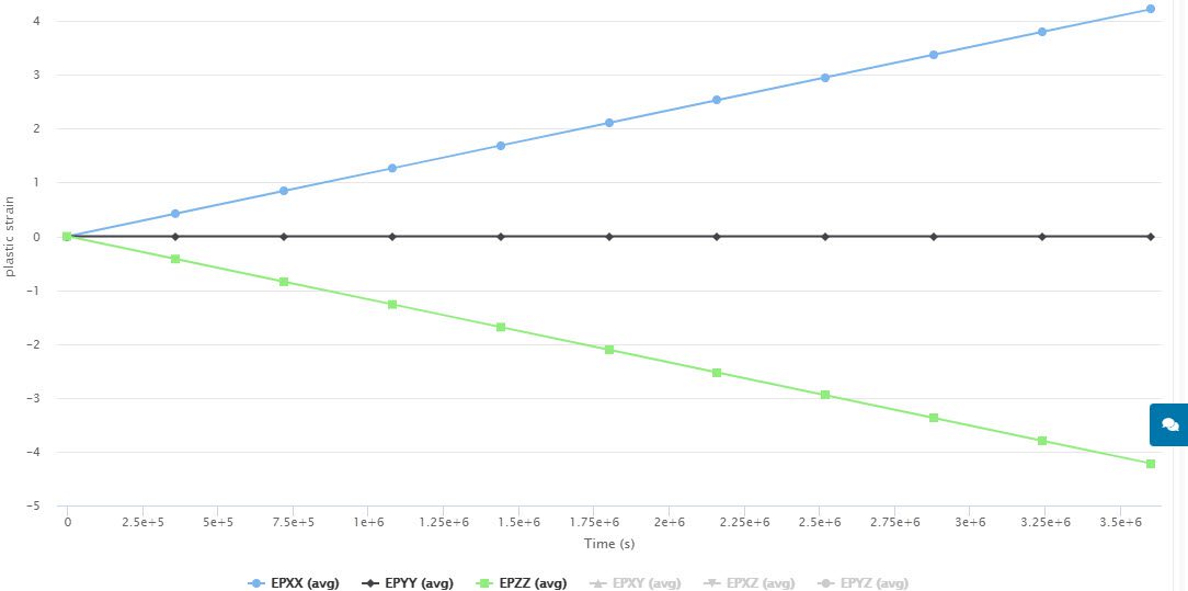
\(\epsilon_{yy}^c\) and \(\epsilon_{zz}^c\) also show very good agreement with the analytical solution, having an error of 0% and 0.0178%, respectively.
Last updated: November 29th, 2023
Did this article solve your issue?
How can we do better?
We appreciate and value your feedback.


