Validation Case: 3D Triaxial Load Primary Creep (NAFEMS Test 11)
This triaxial load primary creep validation case belongs to solid mechanics. This test case aims to validate the following parameters:
- Creep material behavior.
- Standard and reduced integration elements.
- Automatic time stepping.
The simulation results of SimScale were compared to the analytical results derived from [NAFEMS_R27]\(^1\).
Geometry
The geometry consists of a cube with an edge length \(l\) = 0.1 \(m\).
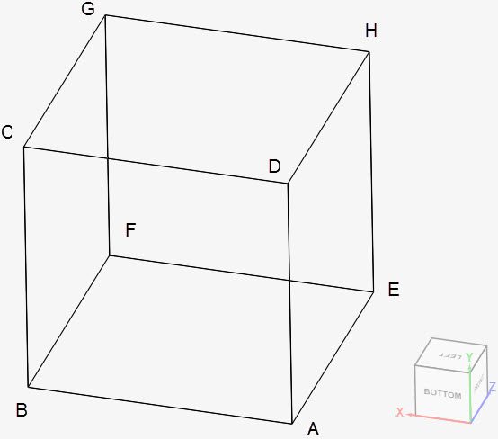
The coordinates for the points in the cube geometry are as tabulated below:
| A | B | C | D | E | F | G | H | |
| x | 0 | 0.1 | 0.1 | 0 | 0 | 0.1 | 0.1 | 0 |
| y | 0 | 0 | 0.1 | 0.1 | 0 | 0 | 0.1 | 0.1 |
| z | 0 | 0 | 0 | 0 | 0.1 | 0.1 | 0.1 | 0.1 |
Analysis Type and Mesh
Tool Type: Code Aster
Analysis Type: Nonlinear static
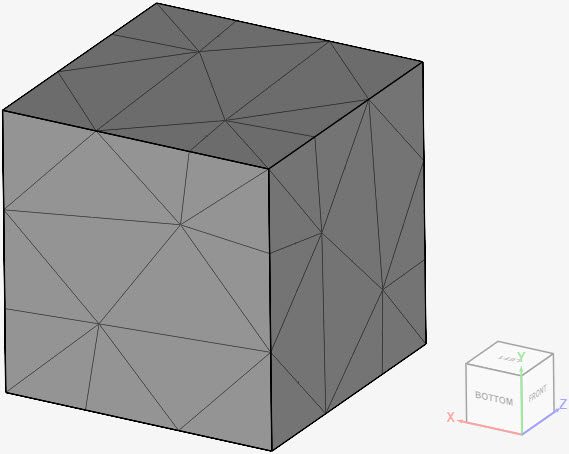
Mesh and Element Types: The mesh used in cases A and B was created using the standard algorithm within SimScale. The same mesh is used in both cases – the only difference between the runs is the element technology integration. Table 2 shows more details about the cases.
| Case | Mesh Type | Number of Nodes | Element Type | Element Technology |
| (A) | Standard | 235 | 2nd order tetrahedral | Standard |
| (B) | Standard | 235 | 2nd order tetrahedral | Reduced integration |
Find below the mesh used for cases A and B. It’s a standard mesh with second-order tetrahedral cells.
Simulation Setup
Material:
- Steel (linear elastic)
- \(E\) = 200 \(GPa\)
- \(\nu\) = 0.3
- \(\rho\) = 7870 \(kg/m³\)
- Creep formulation: Time hardening
- \(A\) = 2.6041667e-46 \(1/s\)
- \(N\) = 5
- \(M\) = -0.5
Boundary Conditions:
- Constraints
- \(d_x\) = 0 on face ADHE;
- \(d_y\) = 0 on face ABFE;
- \(d_z\) = 0 on face ABCD.
- Surface loads
- \(t_x\) = 300 \(MPa\) on face BCGF;
- \(t_y\) = 200 \(MPa\) on face CDHG;
- \(t_z\) = 100 \(MPa\) on face EFGH.
Advanced Automatic Time Stepping:
The following advanced automatic time stepping settings were defined under simulation control:
- Retime event: field change;
- Target field component: internal variable V1 (accumulated unelastic strain);
- Threshold value: 0.0001;
- Time step calculation type: mixed;
- Field change target value: 0.00008.
Reference Solution
The equations used to solve the problem are derived in [NAFEMS_R27]\(^1\). As SimScale uses SI units, the reference solution was adopted to a time unit of seconds instead of hours.
$$\epsilon_{xx}^c = – \epsilon_{zz}^c = \frac{0.004218}{60} \sqrt{t} \tag{1}$$
$$\epsilon_{eff}^c = \frac{0.004871}{60} \sqrt{t} \tag{2}$$
$$\epsilon_{yy}^c = 0.0 \tag{3}$$
Result Comparison
Find below a comparison between SimScale’s results and the analytical solution presented in [NAFEMS_R27]\(^1\) for the average creep strain \(\epsilon_{xx}^c\) of the cube. The creep time is 3.6e6 \(s\) (equivalent to 1000 hours).
| Case | [NAFEMS_R27] | SimScale | Error (%) |
| (A) | 0.133380 | 0.133107 | -0.205 |
| (B) | 0.133380 | 0.133107 | -0.205 |
In Figure 3, we can see how \(\epsilon_{xx}^c\), \(\epsilon_{yy}^c\), and \(\epsilon_{zz}^c\) are evolving for case B.
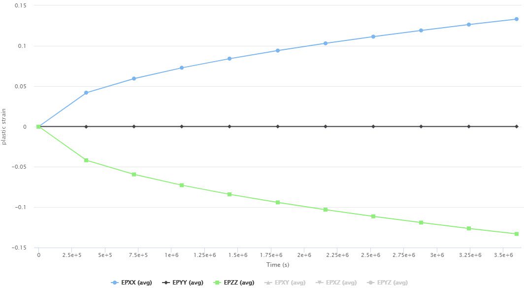
\(\epsilon_{yy}^c\) and \(\epsilon_{zz}^c\) also show very good agreement with the analytical solution, having an error of 0% and -0.205%, respectively.
Last updated: November 29th, 2023
Did this article solve your issue?
How can we do better?
We appreciate and value your feedback.