Surface heat flux
With the surface heat flux boundary condition, a prescribed constant or variable heat flux per unit area can be applied to the assigned boundary faces. This is useful to model heat sources or heat sinks, where the power per unit area is known.
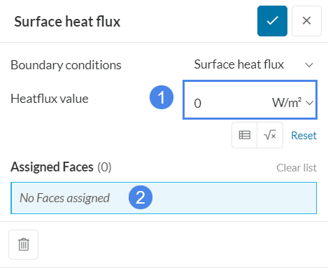
The parameters of the boundary condition are:
- Heat flux value: The value of the surface heat flux variable to be applied, in units of power \((W, Btu/s)\) per units of area \((m^2, in^2)\).
- Assignment: Set of faces where the heat flux value will be applied.
Application Hints
For positive flux values, the heat enters the body (heat source), and for negative values the heat leaves the body (heat sink).
Supported Analysis Types
The following analysis types support the usage of this boundary condition:
Resultant Heat Transfer
The heat transfer on each element of the assigned surfaces will be given by:
$$ \kappa (\nabla T \cdot \vec{n}) = Q_s $$
Where:
- \( \kappa \) is the thermal conductivity of the material,
- \( \nabla T \) is the local temperature gradient,
- \( \vec{n} \) is the area normal vector of the element boundary surface, and
- \( Q_s \) is the specified surface heat flux.
Variable Heat Flux
Variable heat flux values can be specified with the use of the formula or table inputs. The allowed functions are:
- Time-dependent: The heat flux varies with respect to time (variable t) in a transient heat transfer, nonlinear static or dynamic thermomechanical simulation. This is useful, for instance, to ramp up the load from zero in nonlinear simulations, where a sudden application of load leads to numerical divergence, or to define power loading curves. This option is available for both formula and table inputs.
- Coordinate-dependent: The heat flux varies with respect to the position in space (variables X, Y, Z). This is useful to apply known power gradients on faces. If the heat flux only depends on 1 variable, both the formula and table input can be used. For 2 or 3 coordinate dependency, only the definition by a formula is allowed.
- Coordinate and time-dependent: The heat flux varies with respect to position in space and time (variables X, Y, Z, t). This option will be available for transient heat transfer, nonlinear static or dynamic thermomechanical simulation. This input is allowed for both formula and table inputs.
- Temperature-dependent: Available in nonlinear simulations, the local heat flux at each point is a function of the surface temperature. This type of function can be used to model radiation heat transfer using the Boltzmann equation, as exemplified in the validation case ‘Hollow sphere, convection and radiation‘, linked below. This option is only available through table input.
Maximum Number of Table Parameters
The underlying structural solver (Code_Aster) supports table function definitions of one or four variables. If you need to define a function of two or three spatial coordinates (X, Y, Z), or even combine it with time, you must create an analytical formula for it.
Related Documentation
- Validation Case: Hollow Sphere, Convection, and Radiation.
- Validation Case: Thermal Effects in High Power LED Packaging.
Last updated: February 13th, 2025
Did this article solve your issue?
How can we do better?
We appreciate and value your feedback.


