Passive Scalar Sources
Passive scalar is a scalar quantity that is not actively involved in the flow physics of the CFD simulation. This is only ensured if the passive scalar source can be considered as a fluid with contaminants/species present in low concentration, getting transported with the fluid flow, thereby having a negligible effect on the thermophysical properties of the fluid.
Hence, passive scalar sources can be used to model the propagation of species like smoke from a burning car in a garage, transport of oxygen within a water flow, or the diffusion of dust or pollutants in a tunnel. Another possible application of passive scalars is to model the mean age of a fluid, for example, air freshness analysis in a meeting room.
It is important to note that, scalar transport does not assume any physical dimensions for passive quantities.
Creating a Passive Scalar Source
- Currently, Passive scalar sources can only be added in the Incompressible Fluid Flow, Conjugate Heat Transfer, and Convective Heat Transfer analysis types.
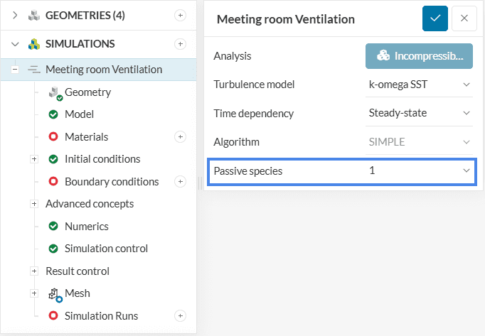
- To create a passive scalar source, first, add one or more Passive species to the simulation setup by going to your simulation project.
Next Steps
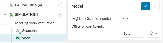
- Navigate to Model in the simulation tree to specify the turbulent Schmidt number and the diffusion coefficient for each passive scalar. Read more about them here.
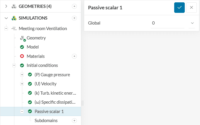
- Under Initial Conditions, you should see a new entry Passive scalar. Keep its value at default Global 0.
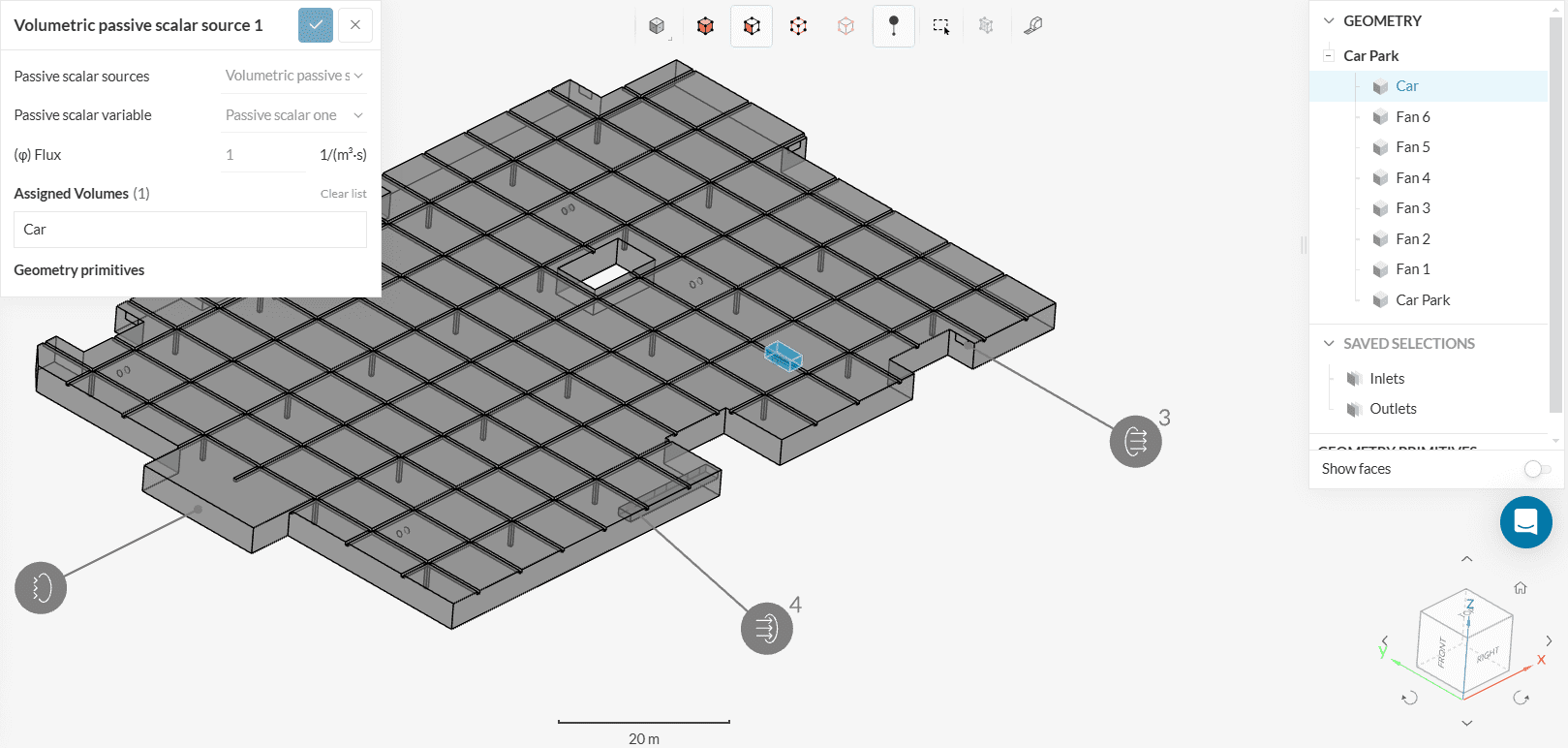
- In the simulation tree, navigate to Advanced Concepts and click on ‘+’ to add a Passive Scalar Source.
The setup looks as shown in Figure 4:
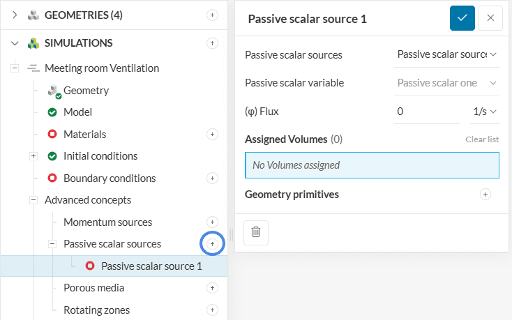
- The passive scalar source can be assigned to a geometry primitive (cartesian box, sphere, cylinder, and point) or by directly assigning the CAD volumes.
Note
Passive scalar sources can also be assigned to faces of the simulation domain. This can be done while assigning boundary conditions. Check our knowledge base article for more details.
Types of Passive Scalar Sources
Two types of passive scalar sources are currently supported:
Passive Scalar Source
This type of source is defined by a flux, which may be interpreted as a concentration per unit time. In other words, it is the rate of change of the passive scalar, given by \(1/s\). The user needs to specify the flux value and select the source region. When using point/s as a geometry primitive each point will bear the concentration equivalent to
$$\phi\times \frac{V_i}{V}$$
Where,
- \(\phi\) = specified flux value \([1/s]\)
- \(V_i\) = volume of cell accompanying the individual point \([m^3]\)
- \(V\) = sum of all cell volumes accompanying all points \([m^3]\) (same as \(V\) for single point)
Volumetric Passive Scalar Source
This type of source is defined by a flux per unit volume. Consequently, the actual flux is implicitly computed using the volume of the source region assigned. The flux is specified in \(1/m^3s\) or \(1/in^3s\). When using point/s as a geometry primitive the concentration is considered for the volume of the cell accompanying the point.
$$\phi\times{V_i}$$
Where,
- \(\phi\) = specified flux value \([1/m^3s]\)
- \(V_i\) = volume of cell accompanying the individual point \([m^3]\)
Note
It is important to understand the correct interpretation of the units used for passive scalar sources. Since passive scalars do not affect the dynamics of fluid flow, units for passive scalars are independent to the unit system of simulation. Thus one can define a passive scalar flux as 100 \(1/s\) and interpret it as a flux of 100 \(g/s\) or 100 \(kg/s\) as per one’s convenience. However, these interpreted units must be kept consistent throughout the simulation setup (for values specified in initial conditions, boundary conditions etc). The scale of the results will directly correspond to the absolute value of input variables.
Example 1
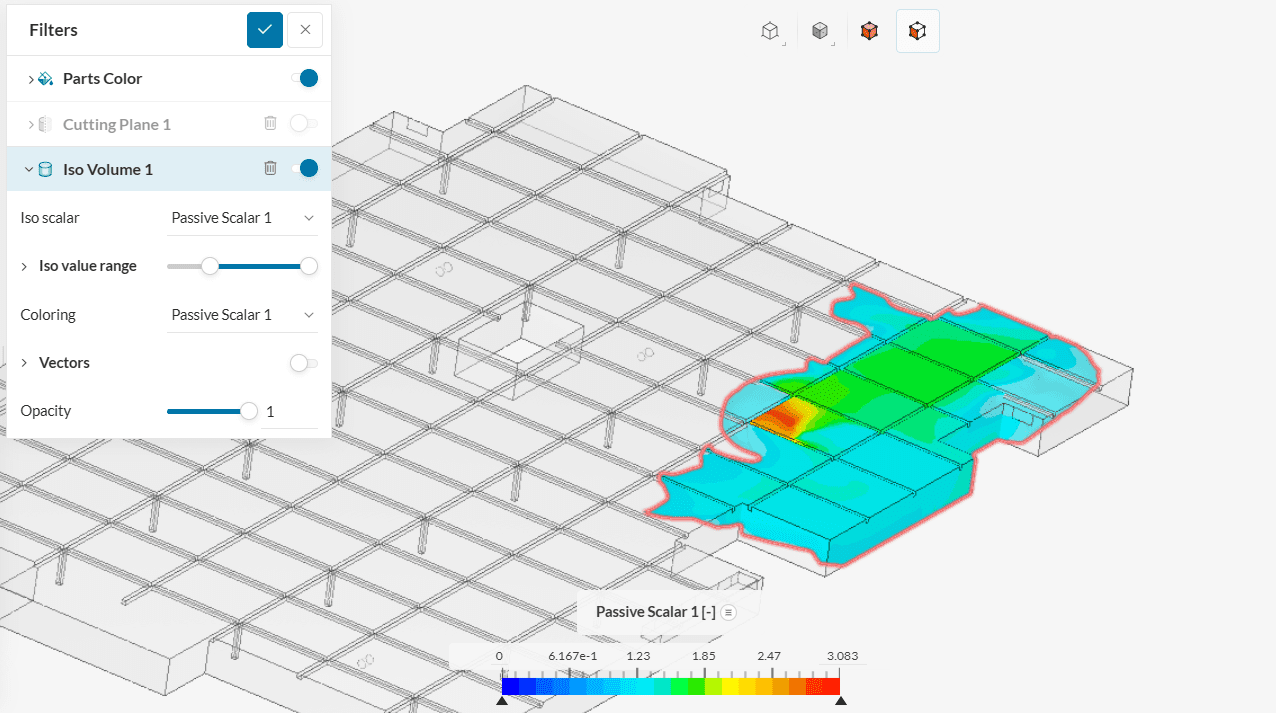
Consider the example of a car park with the car modeled as a box. The intention here is to control the CO (Carbon monoxide) contamination by simulating the CO as a passive scalar coming out of the car acting as a source. Hence, we define this car as a passive scalar source with a volumetric flux of 1 \(\frac{1}{m^3s}\). This value of ‘1’ can be taken as per your convenience, 1 \([gm]\) per car volume \([m^3]\) per second for example.
Using the Iso volume filter in the SimScale post-processor we can now observe the spread of the CO in the car park emanating from the car to evaluate the contamination caused and deduce conclusions on the safety based on the severity level.
Example 2
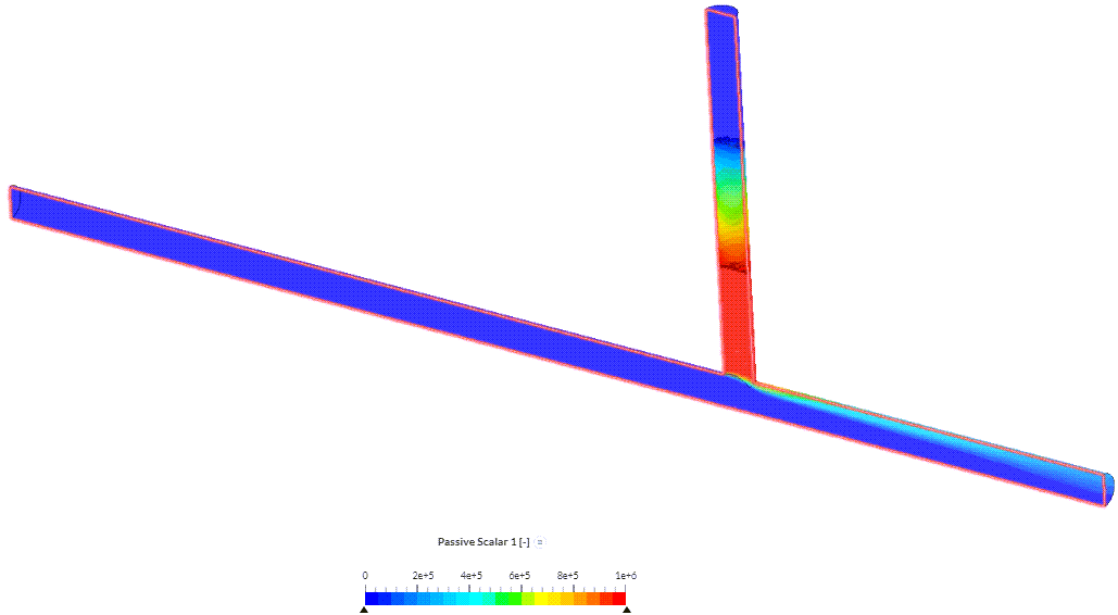
To shed some light on the physical interpretation of passive scalar, especifically on its magnitude within the fluid flow, one can take advantage of the correlation: 1 ppm = 1 mL/m³ = 1 mg/kg. Therefore, if those units are kept consistent throughout the simulation set-up, the passive scalar contour plot can be interpreted in ppm. To ilustrate this, we consider the following pipe junction with a passive scalar source that is supposed to generate 1e6 ppm of scalar.
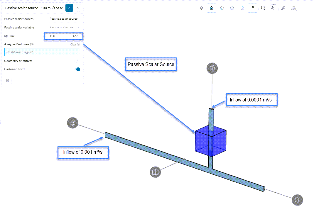
The source is placed in a pipe that has an inflow of 0.0001 m³/s, so the source value [1/s] can be defined by multiplying the 1e6 ppm by the inflow of 0.0001 m³/s, which amounts to 100 mL/s. Here the mL is the “interpretable” unit related to the numerator of 1/s. Since the units are consistent with the correlation aforementioned, the contour plot for the passive scalar can be interpreted in ppm.
It is advised that readers practice the following tutorials in order to get a good grasp of the above concept:
- Carpark Contamination Simulation Using Scalar Transport
- Thermal Comfort Analysis of a Meeting Room
- Contamination of a Power Plant
Last updated: January 22nd, 2026
Did this article solve your issue?
How can we do better?
We appreciate and value your feedback.


