What is a Courant Number?

The intention of this article is to define what a Courant number is and to give a best practice of how to set your mesh and time step in case you have problems with the Courant number. This blog article also contains further details on the CFL condition.

CFL Condition – Courant Number

The Courant–Friedrichs–Lewy or CFL condition is related to the distance that any information travels within the mesh during a time step. The derivation of the CFL condition leads to the following formula for the Courant number:

$$C = u \frac{\Delta t}{\Delta x} \tag{1}$$

where \(C\) is Courant number, \(u\) is velocity magnitude, \(\Delta t\) is time step size and \(\Delta x\) is the length between mesh elements.

The Recommended Courant Number

The Courant number is a dimensionless value representing the number of mesh cells traveled at a given timestep.

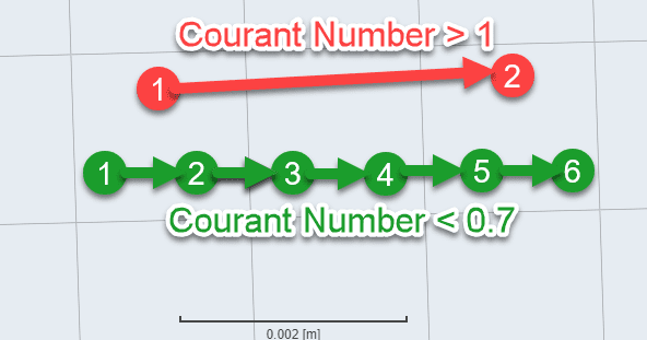
If we imagine a fluid particle in a certain cell of the computational domain, when the Courant number is above 1 the particle may skip the neighbor cells completely after a timestep. Following the same logic, if the Courant number is smaller than 1, the particle is not going to completely skip a neighbor mesh cell after a single timestep. The image below illustrates these scenarios.

In most analysis types, since the time integration schemes used are implicit, using Courant numbers larger than 1 is a possibility from an accuracy/stability perspective. However, for transient multiphase simulations it is highly desirable to keep the maximum Courant number smaller than 1 since an explicit time integration is applied to the phase fraction.

Looking back at the equation 1 above, to decrease the Courant number we can either:

• Decrease the time step \(\Delta t\), or
• Coarsen the mesh i.e. increase \(\Delta x\)

Simulation Setup

Within the simulation control tab, the Adjustable time step entry can be set to True or False. When set to False, the Delta t value will remain constant throughout the entire simulation.

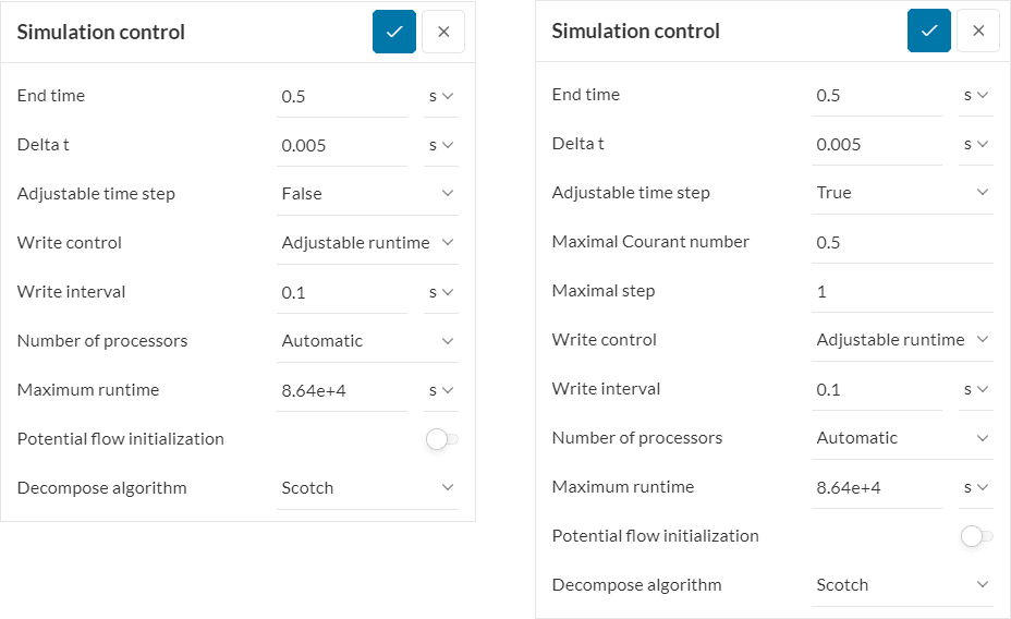
When Adjustable time step is True, the user is prompted to provide the maximal Courant number allowed in the simulation run. With this configuration, the Delta t is used only in the first time step and afterward SimScale will adjust the timestep according to the maximal Courant number allowed.

Best Practices

Certain consideration should be taken into account when choosing a time step or the maximum CFL number in the Simulation Setup tab:

• Accuracy: The temporal discretization error increases with the time step and the resulting CFL number, if the mesh and simulation setup remain constant. Transient effects that are faster than the time step size wont be resolved and the time discretization schemes assume a constant temporal gradient within a time step. As a rule transient effects should be resolved with at least 100 time steps. To quantify the temporal discretization error on a quantity, a study based on 3 simulations resolving the transient effects by, for example, 100, 1000 and 10000 time steps can be performed.
• Stability: Too big time steps and resulting CFL numbers may influence the stability of the simulation and lead to divergence. If the temporal resolution is sufficient for the accuracy, stability can be achieved by performing additional outer iterations. This can be done in the Numerics tab.
• For transient multiphase runs, keep the maximum Courant number smaller than 1. For other analysis types, using a maximum Courant number larger than 1 is possible/desired, as long as the best practices for accuracy and stability (above) are observed
• Even when using the adjustable time step approach, start the simulation with a very small Delta t value. This ensures that the simulation calculates the first steps smoothly.

Example

Taking a multiphase simulation as an example, the Courant number would be optimally kept under 1.

1. Make sure the sizes of the elements in the mesh do not differ too much. Measure the average cell size of your mesh. Let’s consider a case where it is about 1.7e-3 \(m\).
2. Now have a look at your flow velocity, let’s assume it is 30 \(m/s\). Accordingly, the average time a particle stays in one cell is 1.7e-3 / 30 = 5.67e-5 \(s\).
3. This is the basis for defining the time step: To make sure your time is not too high set your initial time step to 10% this calculated value (in our case this would be 5.6e-6 \(s\)).
4. Multiply this time by the number of time steps you want to obtain the value for the end time.