How to Compute the Coefficients for Rayleigh Damping?

The Rayleigh damping model is an approximation to viscous damping available in Harmonic and Dynamic FEA simulations. It allows modeling the energy dissipation in the material due to internal friction, assuming it is proportional to the strain or deformation rate. As such, it is common to be in the need to determine the model coefficients from experimental or assumed data. In this article, we will explore the definition and the methodology to determine the Rayleigh damping coefficients.

Definition:

The damping force term \(F(t)\) is assumed to be proportional to the deformation rate \(\dot{x}\), as seen in the general dynamic motion equation for a one degree of freedom system with inertial mass \(m\), damping coefficient \(c\) and spring stiffness \(k\):

$$ m\ddot{x} + c\dot{x} + kx = F(t) $$

The Rayleigh model approximates the damping coefficient as a linear combination of mass and stiffness:

$$ c = \alpha k + \beta m $$

where \(\alpha\) is stiffness-proportional damping coefficient \([seconds]\) and \(\beta\) is mass-proportional damping \([1/seconds]\).

Substituting into the equation of motion and rearranging in terms of the natural frequency of oscillation \(\omega_n\) and the damping ratio \(\zeta\), we obtain:

$$ \ddot{x} + \frac{c}{m} \dot{x} + \frac{k}{m} x = \frac{F(t)}{m} $$

$$ \ddot{x} + 2 \zeta \omega_n \dot{x} + \omega_n^2 x = \frac{F(t)}{m} $$

Where,

$$ \omega_n^2 = \frac{k}{m} $$

$$ \zeta = \frac{c}{c_{critic}} = \frac{c}{2m\omega_n} $$

Then we can relate the Rayleigh damping coefficients to the damping ratio:

$$ \zeta = \frac{1}{2 m \omega_n}(\alpha k + \beta m) $$

$$ \zeta = \frac{1}{2}\bigg( \alpha \omega_n + \frac{\beta}{\omega_n} \bigg) $$

From this equation we can see that the Rayleigh model can reproduce three cases:

Damping is Proportional to the Inertia

In this case, the stiffness coefficient \(\alpha = 0\) and thus:

$$ \zeta = \frac{ \beta }{2 \omega_n } $$

For a given constant value of \(\beta\), it is seen that the damping is inversely proportional to the natural frequency, as shown in the illustration:

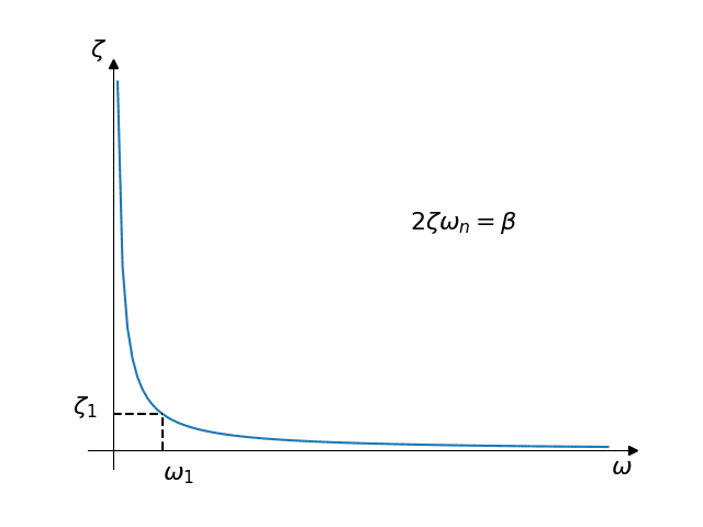
Moreover, if one computes \(\beta\) from the damping ratio \(\zeta_1\) at a given natural frequency \(\omega_1\), all the natural frequencies below it will be amplified and the frequencies above it will be attenuated. The effect is more dramatic the farther the frequencies are from the reference value.

Damping is Proportional to the Stiffness

In this case, the mass coefficient \(\beta = 0\) and thus:

$$ \zeta = \frac{1}{2} \alpha \omega_n $$

It is seen that, contrary to the first case, here the damping is directly proportional to the natural frequency:

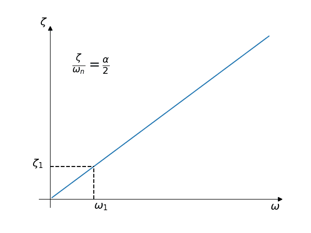
If one computes \(\alpha\) from the damping ratio \(\zeta_1\) at a given natural frequency \(\omega_1\), then the natural frequencies below will be attenuated and the frequencies above will be amplified.

General case

In the case of using the model with two parameters, the proportionality of damping against frequency is convex:

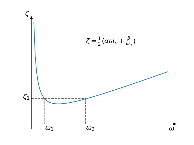
In this case one needs two damping ratios and two natural frequencies to create a pair of equations and solve for \(\alpha\) and \(\beta\). The model gives some flexibility on where to place the natural frequencies, but in general, frequencies too far away from the ones used in the computation will be amplified.

In the particular case of using equal damping ratios for the two frequencies, it is important to note that the damping ratio will not be constant inside the range defined by the sample points, but the inner frequencies will be attenuated. That is, the inner frequencies will have a lower damping ratio.

Computing the Rayleigh Damping Coefficients

In the most common case, a transient response curve from the system is obtained and the damping ratio \(\zeta_1\) is determined for the lowest natural frequency \(\omega_1\) by measuring the (logarithmic) attenuation of successive peaks:

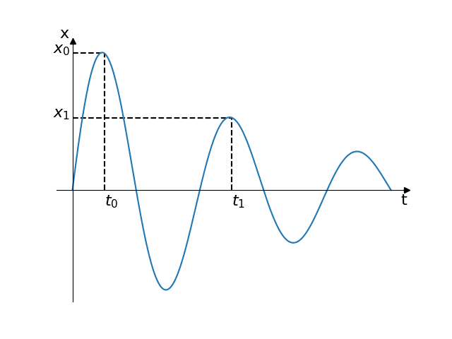
$$ \zeta = \frac{ \delta }{ \sqrt{ \delta^2 + (2\pi)^2 }} $$

$$ \delta = \ln{ \frac{ x_0 }{ x_1 } } $$

$$ f = \frac{1}{T} = \frac{1}{t_1 – t_0} $$

$$ \omega = 2 \pi f $$

It is then most common to assume the case of damping proportional to the stiffness, that is, \(\beta= 0\), and the \(\alpha\) stiffness coefficient is computed from:

$$ \alpha= \frac{ 2 \zeta_1 }{ \omega_1 } = \frac{ \zeta_1}{ \pi f_1} $$

If the knowledge on the system indicates the case of damping decreasing with the frequency, then one can assume the case of damping proportional to the inertia, where \(\alpha = 0\) and determine the mass coefficient \(\beta\):

$$ \beta = 2 \zeta_1 \omega_1 = 4 \pi \zeta_1 f_1$$

If there is not such test data or knowledge of the system, or if one wish to apply an approximate damping ratio over a range of frequencies, then we can use the general case and build a system of two equations:

$$ \zeta_1 = \frac{1}{2} \bigg( \alpha \omega_1 + \frac{\beta}{\omega_1} \bigg) $$

$$ \zeta_2 = \frac{1}{2} \bigg( \alpha \omega_2 + \frac{\beta}{\omega_2} \bigg) $$

Then solve for the unknown coefficients, keeping in mind the considerations given above for the general case and the influence of the model on natural frequencies inside and outside the range of interest. That is, perhaps one wants to achieve a mean damping ratio over the range, then compensate the attenuation by modifying the input damping ratios, or by performing some least-squares approximation from more than two frequency points.