Atmospheric Boundary Layer Inlet for Incompressible LBM

The Atmospheric Boundary Layer Inlet is an exclusive boundary condition for the Incompressible (LBM) simulation type. This article will go through the necessary details for the configuration of this boundary condition.

Overview

For external aerodynamic simulations, a common approach is to define a velocity profile at the inlet, where the velocity changes with the height. In Incompressible (LBM), there are two ways to achieve this result:

1. Using a table input with a Velocity inlet boundary condition
2. Using an Atmospheric boundary layer inlet boundary condition

With the first approach, the user needs to define a table with the velocity at each height of interest. The second option is a much more automated workflow, which will be explored in the next section.

Atmospheric Boundary Layer Inlet

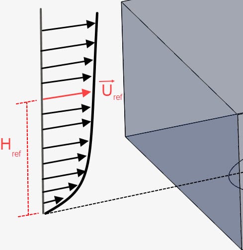
The setup of an atmospheric boundary layer inlet condition is simple. The figure below shows the configuration window:

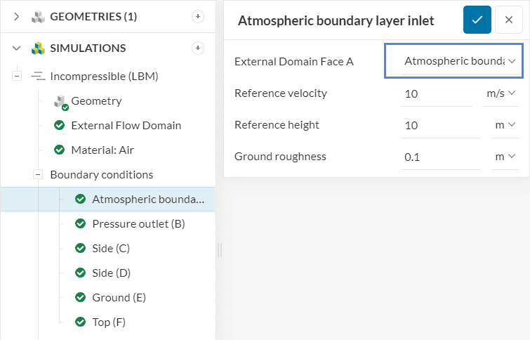
Having Figure 1 in mind, the boundary condition requires the following parameters:

• Reference velocity $u_{ref}$ of the velocity profile
• Reference height, often called $z_{ref}$ or $h_{ref}$, at which the reference velocity is measured. In case there is no terrain, the height is measured as the distance to the bottom of the External Flow Domain or any other no slip wall defined in the simulation setup. Alternatively, if there is a terrain intersecting with the inlet, the height above ground is measured against the terrain surface
• Ground roughness $z_0$, which represents the aerodynamic roughness length. The ground roughness is used to model the effects of vegetation and buildings upstream of the inlet. This documentation page shows the usual values for $z_0$.

Formulation

The formulation described below controls the inlet profile for the velocity $u$, turbulent kinetic energy $k$, and specific dissipation rate $\omega$, based on the user-defined parameters. For organization purposes, a table containing the meaning of each parameter can be found at the end of this section.

The logarithmic velocity profile normal to the inlet has the following formulation:

$$\begin{array}{}\text{(1)}& u=\frac{u^{\ast }}{K}\cdot ln\left(\frac{z+z_0}{z_0}\right)\end{array}$$

The other two velocity components are null. The friction velocity $u^{\ast }$ is given by equation 2:

$$\begin{array}{}\text{(2)}& u^{\ast }=K\cdot \frac{u_{ref}}{ln\left(\frac{z_{ref}+z_0}{z_0}\right)}\end{array}$$

Equation 3 shows the turbulent kinetic energy $k$ expression:

$$\begin{array}{}\text{(3)}& k=\frac{{u^{\ast }}^2}{\sqrt{c_{\mu }}}\end{array}$$

Finally, the specific dissipation rate $\omega$ is given by the expression below:

$$\begin{array}{}\text{(4)}& \omega =\frac{u^{\ast }}{K\cdot \sqrt{c_{\mu }}}\cdot \frac{1}{z+z_0}\end{array}$$

The table below contains a description of all parameters used in equations 1 through 4:

Parameter	Description	Units
$u$	Velocity component, normal to the inlet	$m/s$
$u^{\ast }$	Friction velocity	$m/s$
$K$	von Karman constant, equal to 0.41	–
$z$	Height (normal to the ground)	$m$
$z_0$	Aerodynamic roughness length (user-defined)	$m$
$z_{ref}$	Reference height (user-defined)	$m$
$u_{ref}$	Reference velocity (user-defined)	$m/s$
$k$	Turbulent kinetic energy	$m^2/s^2$
$c_{\mu }$	Turbulent viscosity constant, equal to 0.09	–
$\omega$	Specific dissipation rate	$1/s$

Expected Result

As an example, let’s use the city block model from this incompressible LBM tutorial. The configuration of the boundary condition is straightforward:

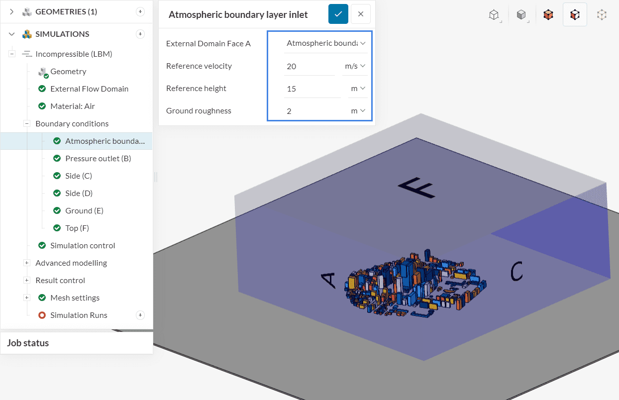
In the example above, a Ground roughness of ‘2’ was defined, since the surroundings of the computational domain consist of a dense urban area.

When post-processing the simulation run, the resulting boundary layer is visible:

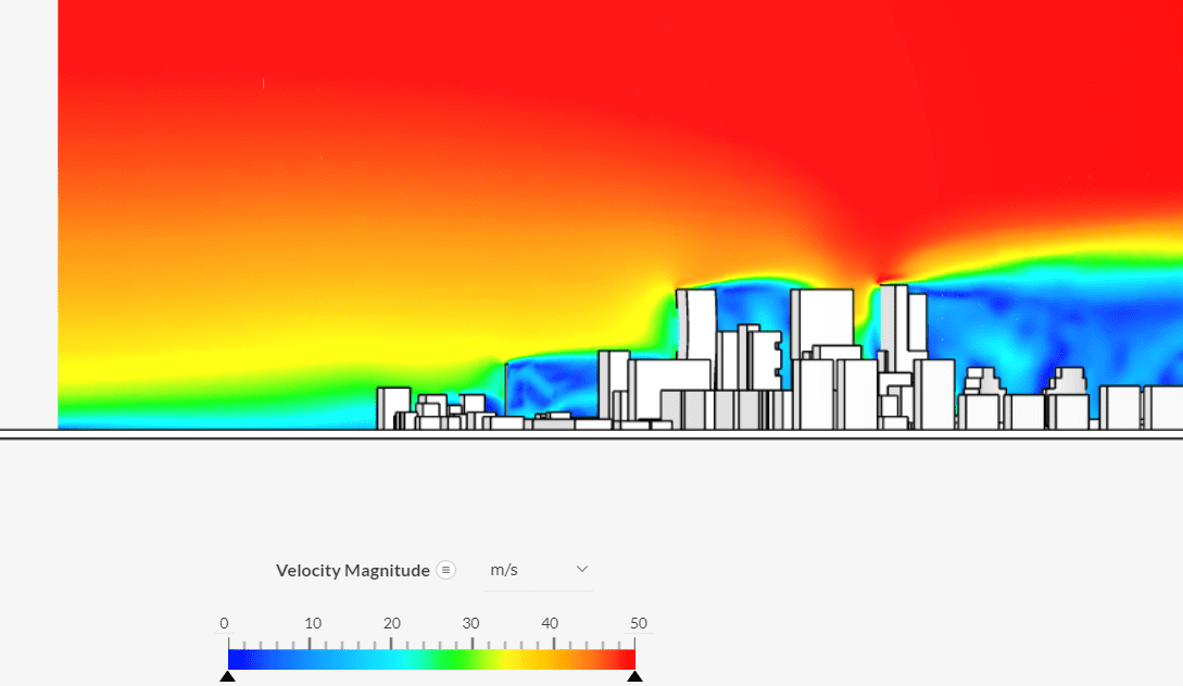
This workflow allows the user to effortlessly define a velocity profile for the inlet, which is optimal for external aerodynamic applications.