Documentation
The scalar transport in a T-junction pipe validation case belongs to fluid dynamics. This test case aims to validate the following:
In this project, a T-junction pipe is used to simulate passive scalar mixing. The SimScale results are compared to the experimental results reported in [1] and [2].
The geometry consists of a pipe with 3 sections: a main pipe, a branch pipe, and a mixing pipe. Figure 1 highlights the pipe dimensions:
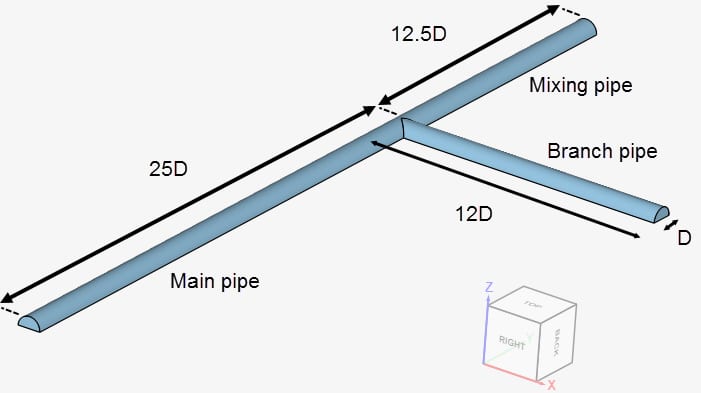
Due to the symmetrical nature of the geometry, only half of the pipe is captured. The pipes have a diameter \(D\) of 51 \(mm\), which is the same as used in the experimental setup. Details of the pipe dimensions are provided in Table 1:
| Dimension | Measurement \([m]\) |
| Diameter of the pipes \((D)\) | 0.051 |
| Length of the main pipe | 1.275 |
| Length of the branch pipe | 0.612 |
| Length of the mixing pipe | 0.6375 |
Tool Type: OpenFoam®
Analysis Type: Incompressible
Turbulence Model: k-omega SST
Mesh and Element Types: This validation case uses a total of 3 meshes, to perform a mesh independence study. All meshes were created in SimScale with the standard mesher algorithm. In Table 2, an outline of the meshes is presented:
| Mesh | Mesh Type | Cells | y+ | Element Type |
| Coarse | Standard | 876174 | < 1 | 3D tetrahedral/hexahedral |
| Moderate | Standard | 1246164 | < 1 | 3D tetrahedral/hexahedral |
| Fine | Standard | 2034350 | < 1 | 3D tetrahedral/hexahedral |
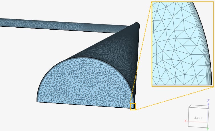
Figure 2 shows the discretization of the mixing pipe obtained with the fine mesh. A total of 10 inflation layers were used to resolve the boundary layer, aiming to achieve a y+ value smaller than 1.
Material:
Boundary Conditions:
Figure 3 will be used as a reference for the definition of the boundary conditions:
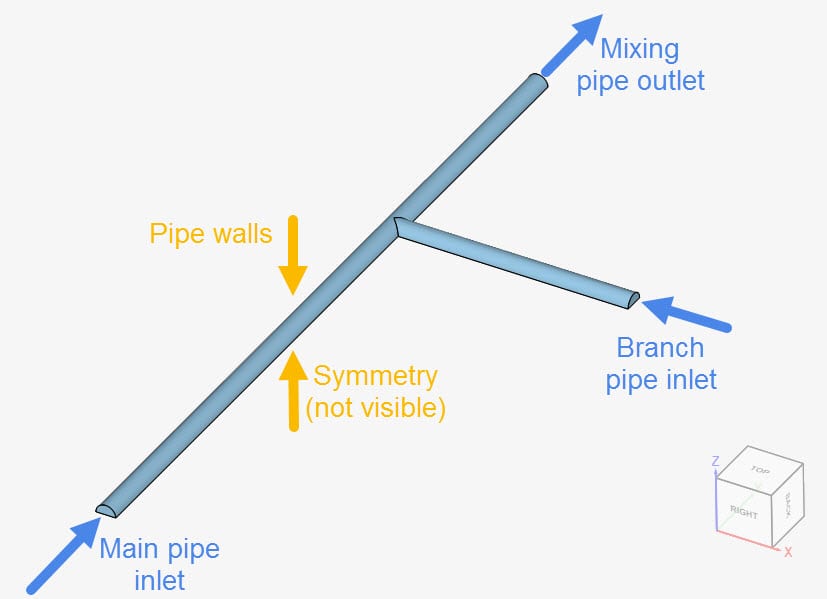
The following boundary conditions are used:
| Boundary | Boundary Type | Velocity \([m/s]\) | Pressure \([Pa]\) | Turb. kinetic energy \([m^2/s^2]\) | Specific dissipation rate \([1/s]\) | Phase Fraction |
| Main pipe inlet | Custom | 0.5 in the y-direction | Zero gradient | Fixed at 9.375e-4 | Fixed at 15.8 | Fixed at 1 |
| Branch pipe inlet | Custom | -0.5 in the x-direction | Zero gradient | Fixed at 9.375e-4 | Fixed at 15.8 | Fixed at 0 |
| Mixing pipe outlet | Custom | Zero gradient | Fixed at 0 | Zero gradient | Zero gradient | Zero gradient |
| Pipe walls | Custom | Fixed at 0 | Zero gradient | Full resolution | Full resolution | Zero gradient |
| Symmetry | Symmetry | Symmetry | Symmetry | Symmetry | Symmetry | Symmetry |
Model:
Note
The turbulent Schmidt number is the ratio of momentum diffusivity to mass diffusivity in a turbulent flow\(^3\).
Following the turbulent Schmidt number sensitivity tests performed by Frank et. al\(^2\), we will use a value of 0.1 in the simulations.
The numerical simulation results for the mixing scalar are compared with experimental data provided by the Laboratory for Nuclear Energy Systems, Institute for Energy Technology (ETHZ), Zürich\(^1\), and also mentioned by Frank et. al\(^2\).
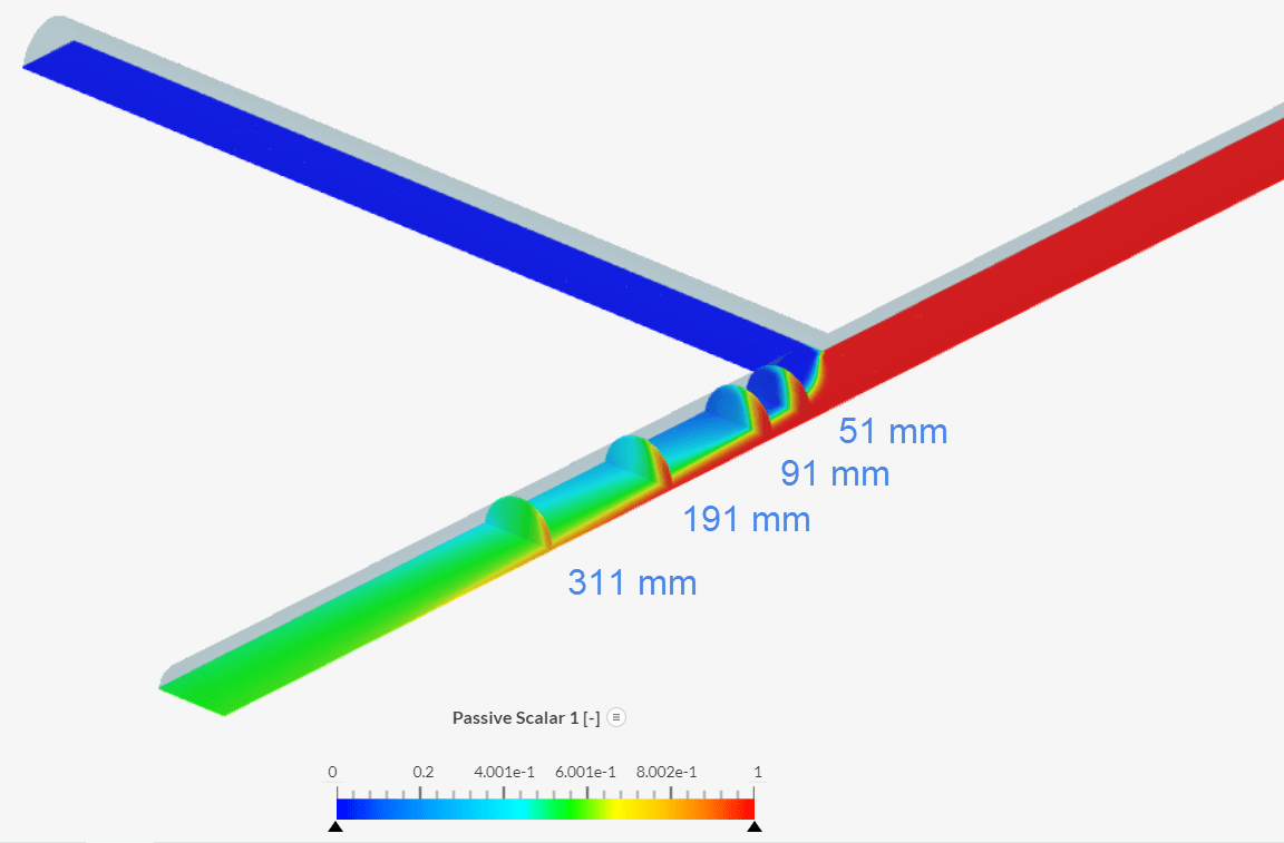
A comparison of the mixing scalar distribution obtained with SimScale and experimental results is presented. The scalar distribution is assessed over four lines, placed 51, 91, 191, and 311 \(mm\) downstream of the T-junction:
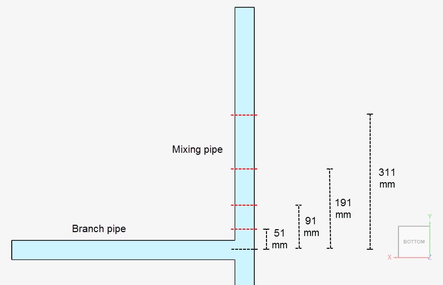
Below, a series of figures show the comparison of results from SimScale to the experimental data for the scalar distribution.
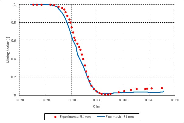
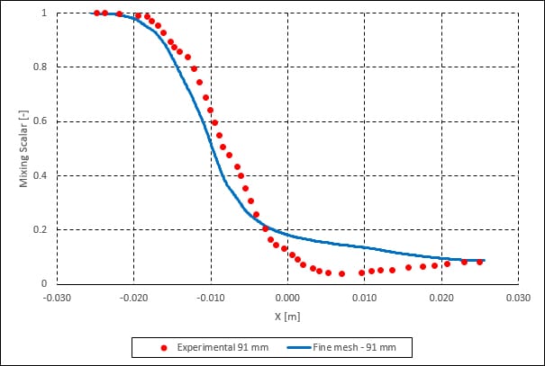
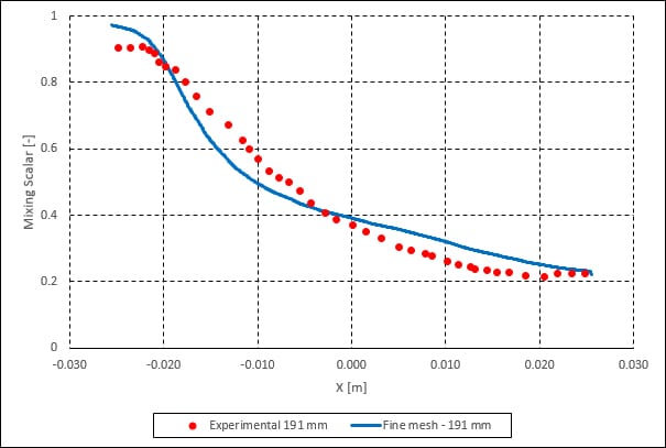
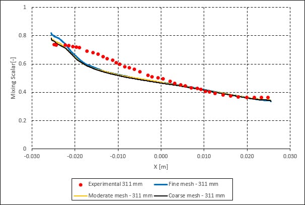
The SimScale results show a good agreement with the experimental data from [1]. Also, a great agreement is observed when comparing the SimScale results to the numerical studies presented by Frank et. al.
References
Last updated: June 17th, 2024
We appreciate and value your feedback.
Sign up for SimScale
and start simulating now