Documentation
This validation case belongs to fluid mechanics, representing the aerodynamics of the Ahmed body study. The aim of this test case is to validate the following parameters:
The simulation results of SimScale were compared to the experimental data presented in [Ahmed]\(^1\).
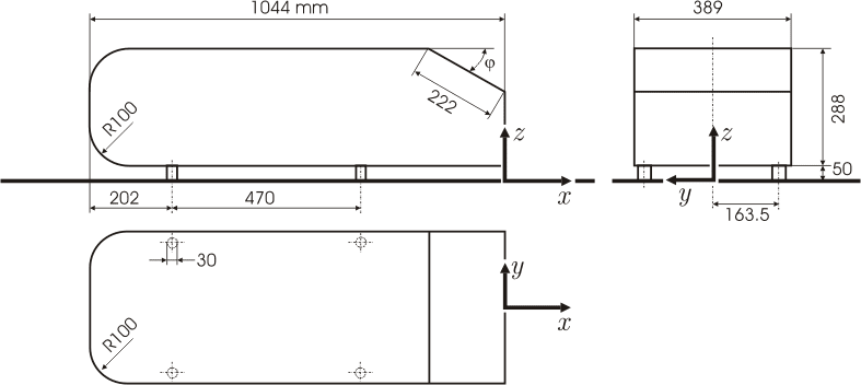
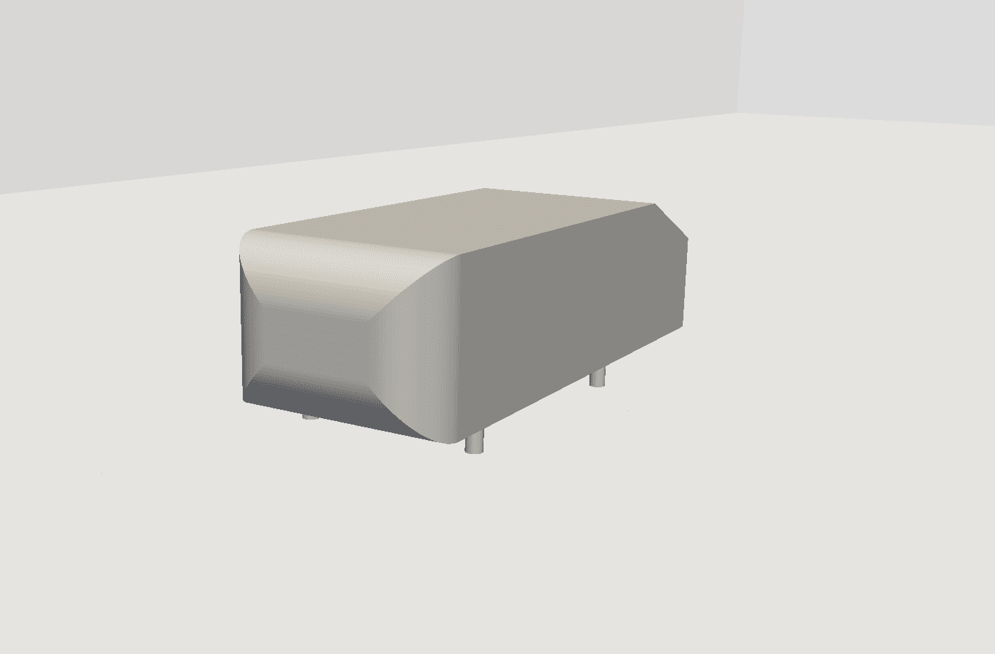
The geometry is created based on the simplified aerodynamic body used by Ahmed et al\(^1\). See Figure 1 for dimensions and Figure 2 for the geometry. The slant angle (\(\phi\)) is set to 25°. The body is placed in a wind tunnel 6 \(m\) x 5 \(m\) x 13.5 \(m\) in order to limit the aerodynamic blockage effect.
Tool Type: OpenFOAM®
Analysis Type: Turbulent Incompressible fluid flow
Mesh and Element Types:
| Mesh | Mesh Type | Number of Cells |
|---|---|---|
| Mesh 1 | Standard | 3,746,887 |
| Mesh 2 | Standard | 6,915,859 |
| Mesh 3 | Standard | 10119321 |
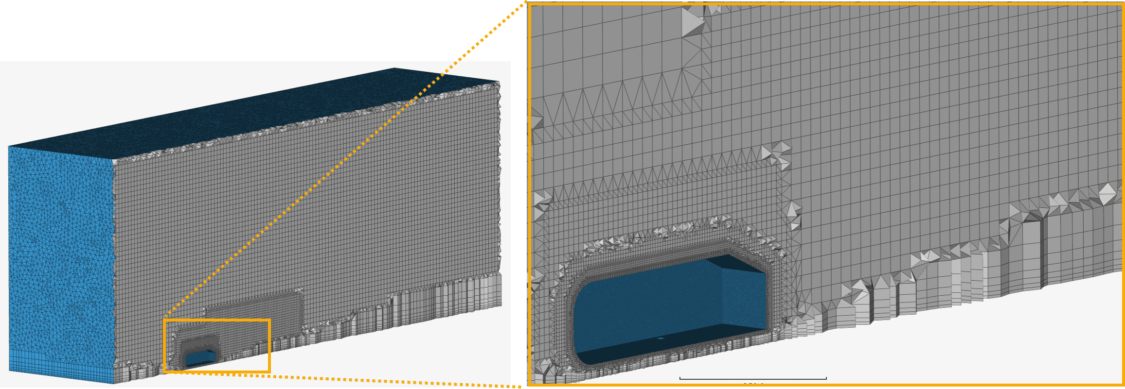
The Standard Mesher algorithm with tetrahedral and hexahedral cells was used to generate the mesh, with refinements near the walls and in the wake region (see Figure 3).
A typical property of the generated mesh is the \(y^+\) (“y-plus“) value, which is defined as the non-dimensionalized distance to the wall, learn more. A \(y^+\) value of 1 would correspond to the upper limit of the laminar sub-layer.
Wall treatment
An average \(y^+\) value of 1 was used for the inflation layer around the body, and 150 for the floor. The \(k-\omega\) SST turbulence model was chosen, with full resolution for near-wall treatment of the flow around the body and with wall function for the floor.
Fluid
Air with a kinematic viscosity of 1.5 x 10⁻⁵ \(kg/ms\) is assigned as the domain fluid.
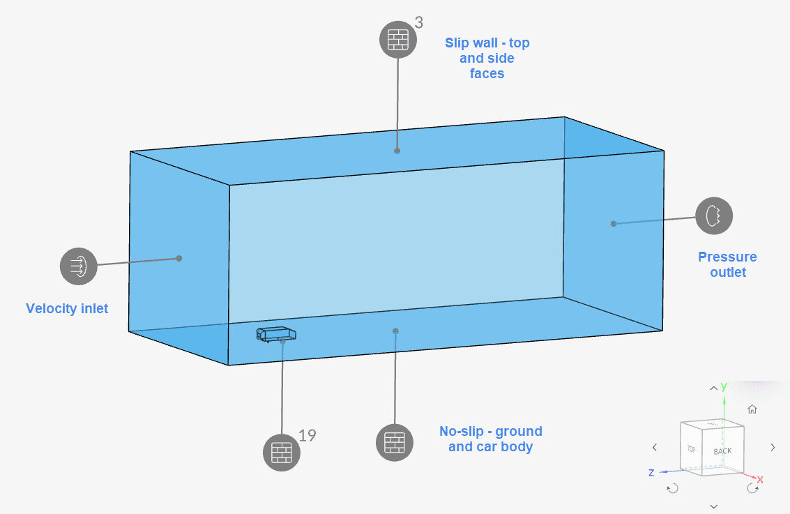
The boundary conditions for the simulation are shown in Figure 4 below:
| Boundary Condition | Face | Value |
| Velocity inlet \([m/s]\) Turb. kinetic energy \([m^2/s^2]\) Specific dissipation rate \([1/s]\) | Inlet | 60 0.135 180.1 |
| Pressure outlet \([Pa]\) | Outlet | 0 (Fixed gauge pressure) |
| Slip wall | Side and top faces | – |
| No slip wall – Wall function | Bottom face (Ground) | – |
| No slip wall – Full resolution | Car body | – |
The free stream velocity of the simulation is 60 \(m/s\), so that the Reynolds number based on the length of the body \(L\) is 4.29e6. Those are the same values presented in the original experiment of Ahmed and Ramm\(^1\).
The experimental solution is presented in Figure 4 in the reference paper\(^1\) giving the value for the drag force coefficient for the slant angle \(\phi\) = 25°:
$$ C_{d} = 0.2875 $$
The drag force is defined as
$$ F_{d}={\frac {1}{2}}\rho \,U^{2}\,C_{d}\,A_x $$
where \(A_x\) (0.115 \(m^2\)) is the projected area of the Ahmed body in the streamwise direction and \(F_{d}\) the drag force. The drag force and drag coefficient were determined by the integration of surface pressure and shear stress over the entire Ahmed body (except for the 4 stilts acting as support).
Mesh #2 was selected due to its accuracy and favorable results in relation to the simulation time. The resulting drag coefficient of the Ahmed body, closest to the reference solution as yielded by Mesh #2, was computed to be 0.2915, which is within a 1.217 % error margin of the measured value.
Table 2 shows the result of the mesh independence study:
| Mesh | DRAG FORCE \([N]\) | DRAG COEFFICIENT | REFERENCE | ERROR [%] |
|---|---|---|---|---|
| Mesh #1 | 73.776 | 0.2985 | 0.2875 | 3.65 |
| Mesh #2 | 72.043 | 0.2915 | 0.2875 | 1.217 |
| Mesh #3 | 70.186 | 0.2835 | 0.2875 | -1.39 |
The difference in the error percentage magnitude between Mesh #2 and Mesh #3 is 0.173, indicating that the drag coefficient values are acceptable.
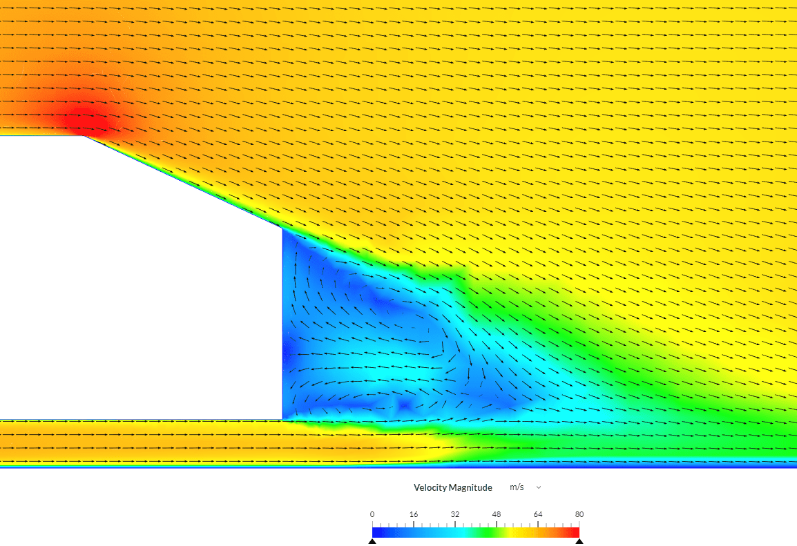
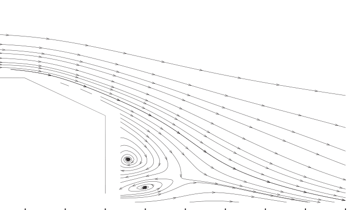
The velocity streamline contour of the mean flow obtained with the simulation is reported in Figure 5, together with experimental results of reference.
Note
If you still encounter problems validating you simulation, then please post the issue on our forum or contact us.
Last updated: August 29th, 2025
We appreciate and value your feedback.
Sign up for SimScale
and start simulating now