Tutorial: Hex-dominant Automated – Internal Flow Through an Angled Pipe
This short tutorial explains how to create a mesh using the automated Hex-dominant operation for internal flow analysis.
Overview
This tutorial teaches how to:
- Mesh with the SimScale Hex-dominant meshing algorithm.
- Inspect your mesh.
Be aware
- This is a tutorial purely about meshing. There will not be a simulation performed.
- The Hex-dominant algorithm is an advanced mesher. If you are new to SimScale and just getting started we highly recommend using the standard mesher.
1. Prepare the CAD Model and Select the Analysis Type
First of all, click the button below. It will copy the tutorial project containing the geometry into your Workbench.
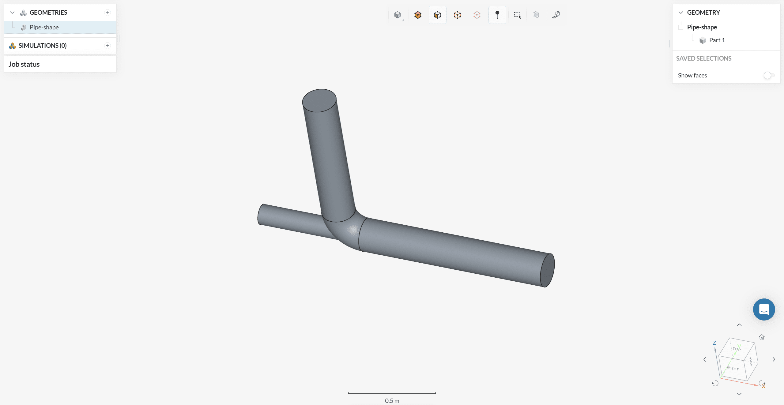
The following picture demonstrates what should be visible after importing the tutorial project.
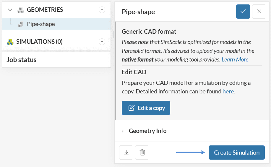
1.1. Create the Simulation
As a first step, we need to create a new simulation. Therefore, left-click on the ‘Pipe-shape’ and then on the ‘Create Simulation’.
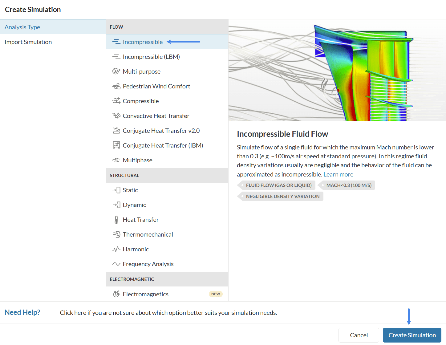
This dialog box allows the user to select the simulation model. Click on the ‘Incompressible‘ option and then on the ‘Create Simulation’ one.
Did you know?
The Hex-dominant meshing algorithm can be used for any flow simulation that is not using the LBM solver, that means:
- Incompressible
- Compressible
- Convective Heat Transfer
- Conjugate Heat Transfer
2. Simulation Setup
In this tutorial, we are going to use the Automatic boundary layers feature from the Hex-dominant meshing tool. With this option, the algorithm automatically creates boundary conditions on all solid walls.
For this feature, it is important to define materials and boundary conditions in advance before generating the meshes.
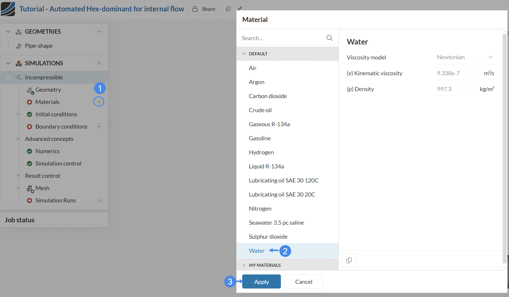
2.1. Materials
To assign a material to the flow region, click on the ‘+ button’ next to Materials. From the list that appears, choose ‘Water’ and press ‘Apply’ to confirm:
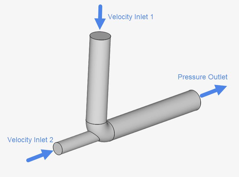
2.2 Boundary Conditions
For this simple pipe simulation, we will set up 3 boundary conditions, as seen below:
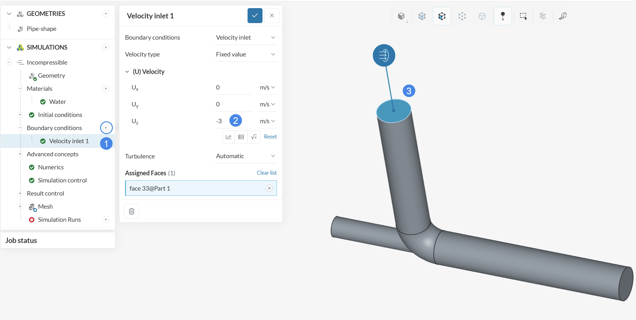
Please click on the ‘+ button’ next to Boundary conditions and select a ‘Velocity inlet’ from the list. Using the orientation cube as a reference, the velocity will be ‘-3’ \(m/s\) in the z-direction, applied to the top face:
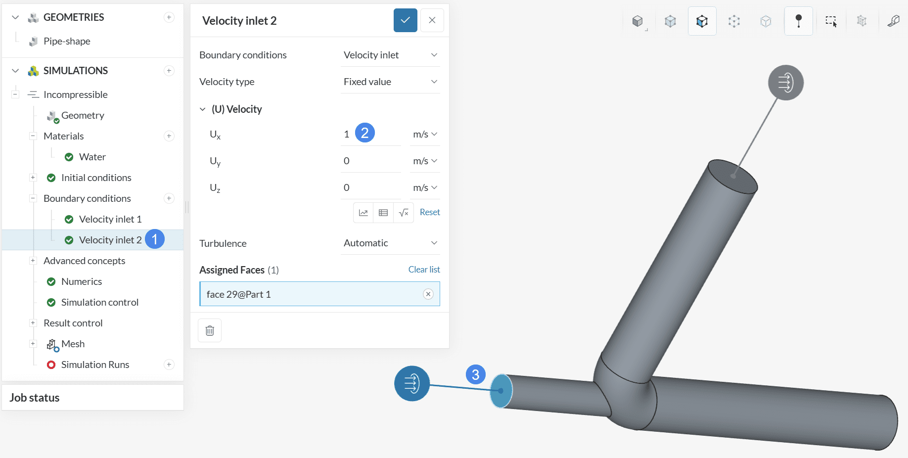
Following the same approach, please define a second velocity inlet boundary condition for the second inlet. This time, the velocity is ‘1’ \(m/s\) in the x-direction:
Finally, please create a new boundary condition – this time a ‘Pressure outlet’, and set it to the outlet face:
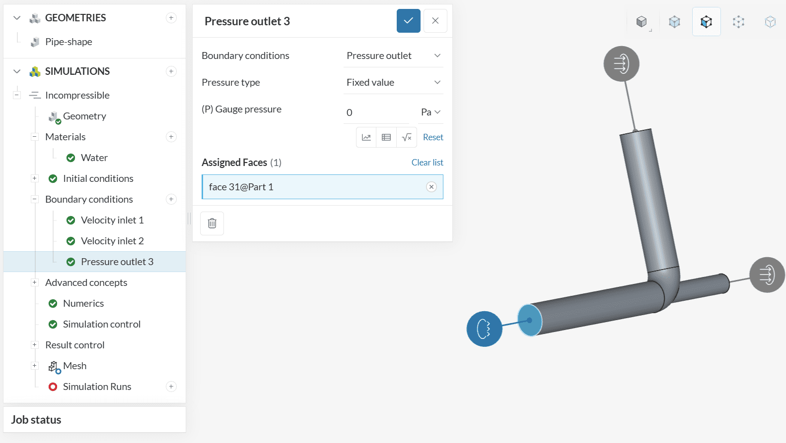
All faces that did not receive an explicit boundary condition are treated as walls. We can now proceed to mesh the geometry.
3. Mesh
We will create five different meshes to demonstrate the differences between the main meshing features available:
- Default Settings
- Global Fineness
- Region Refinement
- Feature Refinement
- Surface Refinement
To access the meshing options click on the ‘Mesh‘ in the simulation setup tree.
3.1 Mesh One: Default Settings
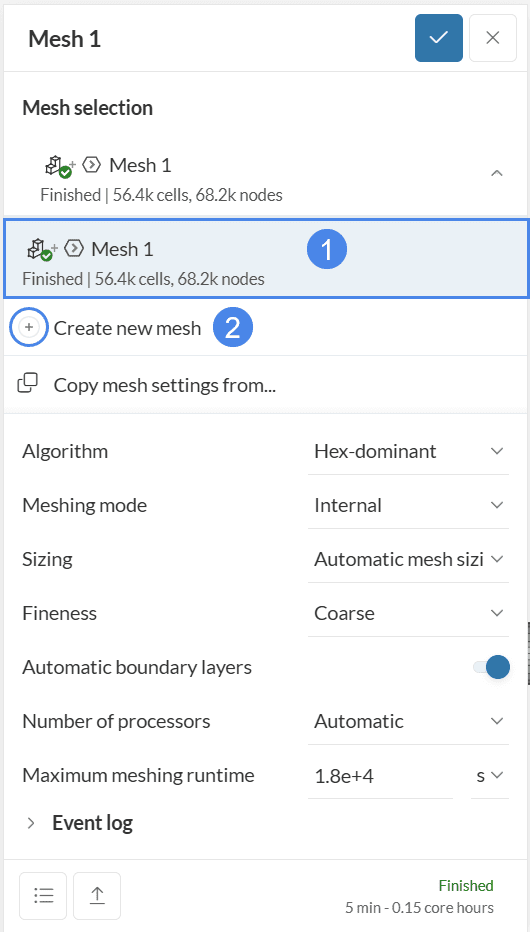
The following picture shows the global mesh settings:
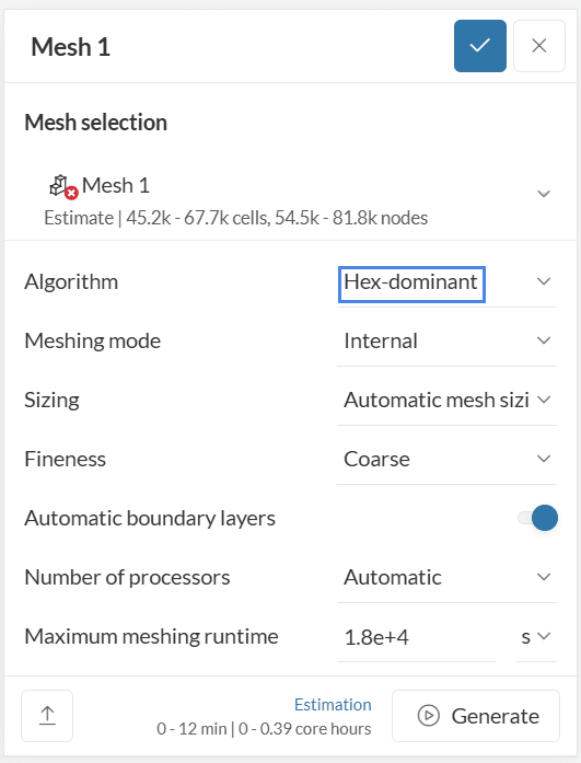
- Choose the ‘Hex-dominant ‘ Algorithm and leave the Meshing mode to its’ original state (‘Internal’).
- Leave the Sizing and Fineness option to their default state.
- The Automatic boundary layers generate layers automatically, based on the boundary conditions set by the user.
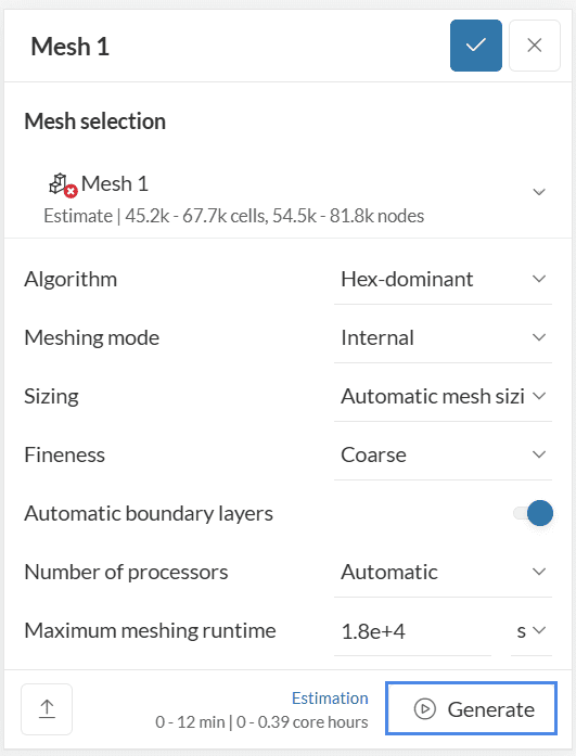
To create a new mesh, click on the ‘Generate‘ option:
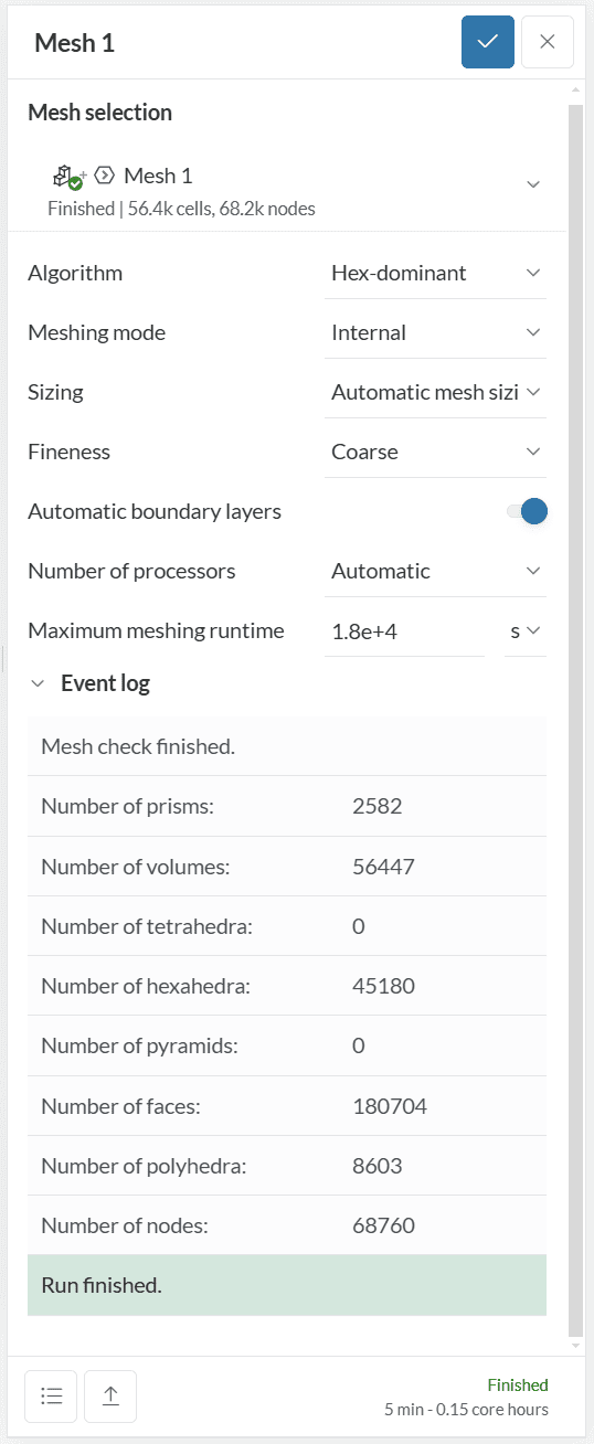
After a couple of minutes, the mesh will be generated. You can see more information about the mesh by clicking on the ‘Event Log‘:
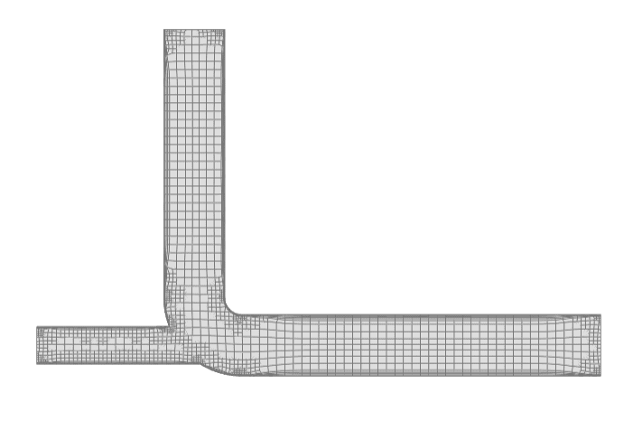
Click on the ‘Mesh clip‘ to inspect the internal mesh. Adjust the settings of the normal. Click on the ‘Generate Mesh Clip‘ icon.
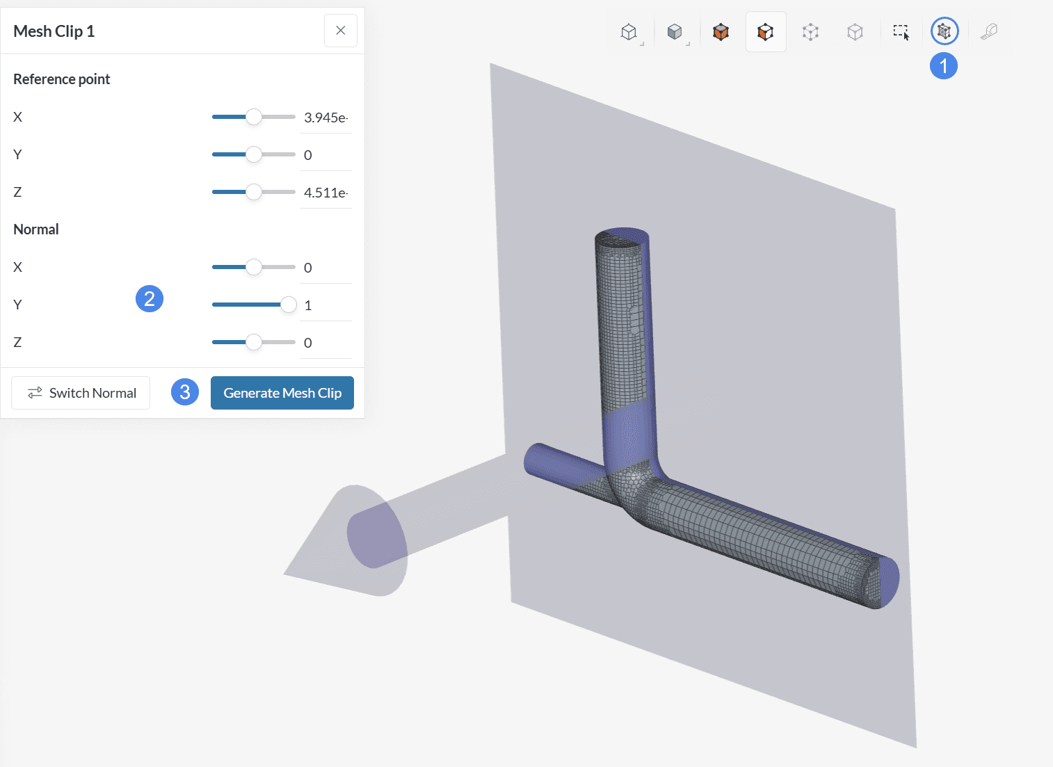
This will appear then on your workbench:
3.2. Mesh Two: Changing Global Fineness
Did you know?
Often, large changes in the mesh’s cell sizes are only spotted in a few regions.
Increasing the global mesh refinements rises the cells drastically.
You can also do this manually, by using one of the local refinement options, foremost being feature, surface, and region refinements.
The settings for the second mesh will be the same, except for ‘Fineness‘.
Follow the steps below to create a new mesh:
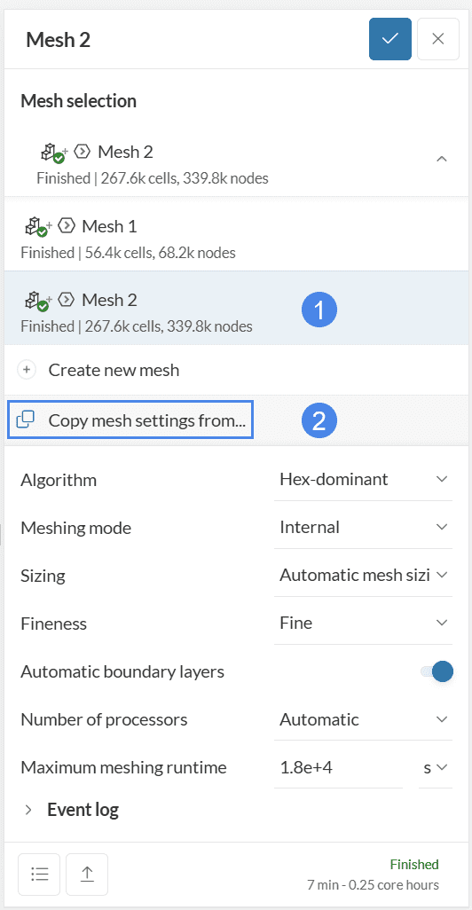
- Click on the current mesh in the main mesh panel.
- Start a new mesh setup by clicking on the ‘+’ icon next to the Create new mesh.
Choose the ‘Hex-dominant‘ algorithm again, then simply change the ‘Fineness‘ level to ‘Fine‘ and ‘Generate‘ the second mesh.
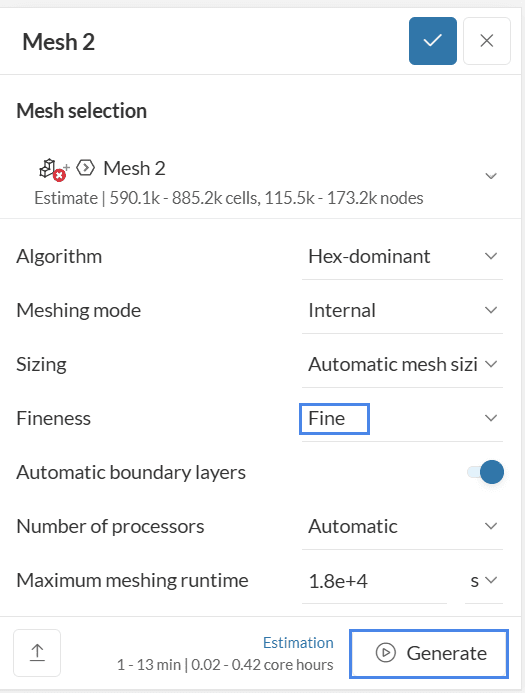
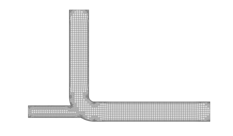
In a few minutes, a finer version of the mesh will be created:
3.3. Mesh Three: Adding a Region Refinement
No refinements were added to the previous cases, but this time, the Region Refinement will be used. Region refinements are assigned to volumes and refine all the cells inside or outside that specific volume.
Depending on the user’s preference, it can refine all volume mesh cells inside the selected volumes up to the specified cell edge length, or the outside volume mesh cells up to the specified cell edge length.
There is also a third mode, accommodating different refinement levels at multiple distances, according to the distance to the surface of the assigned volumes. Start by copying ‘Mesh Two‘. Click on the name of the mesh in the main mesh panel, then select the ‘Copy Mesh settings’. You can choose which already created mesh you want to duplicate by choosing it from a window that will appear.
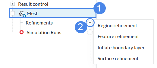
If you want to add any kind of refinements:
- Select the ‘Mesh‘ in the simulation tree.
- Click on the ‘+’ icon next to the Refinements.
- Pick the type of refinement you wish from the menu that will appear.
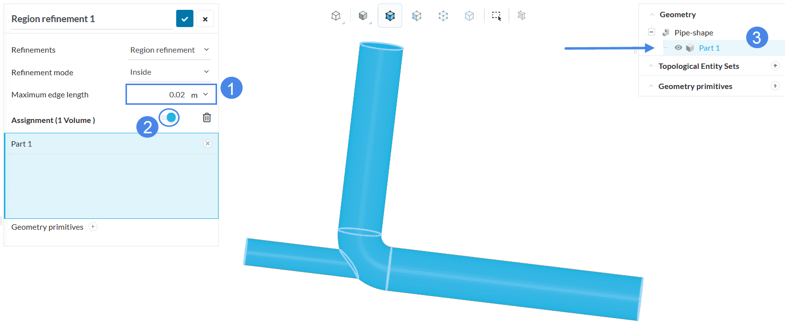
After you pick the ‘Region refinement’, proceed to set the maximum edge length to 0.02 \(m\). Make sure the Assignment is toggled on, and choose the whole part from the geometry tree.
The third mesh, with a region refinement, will be generated after roughly 5 minutes.
3.4. Mesh Four: Adding a Feature Refinement
A feature refinement can be used to refine the geometry’s feature edges. Refinement settings include distance and length. The edge and surface mesh will then be refined up until the specified distance in all directions from the extracted edges. The length parameter determines the intended cell edge length.
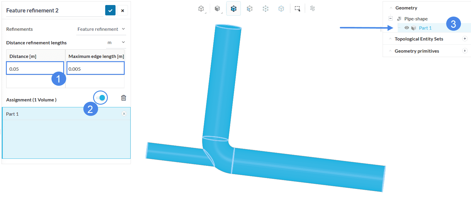
After you copy the mesh settings from Mesh Three pick the ‘Feature refinement’, do the following:
- Set the ‘Distance‘ to 0.05 \(m\) and the ‘Maximum edge length‘ to 0.005 \(m\)
- Make sure the ‘Assignment’ is toggled on.
- Apply the refinement on the whole part.
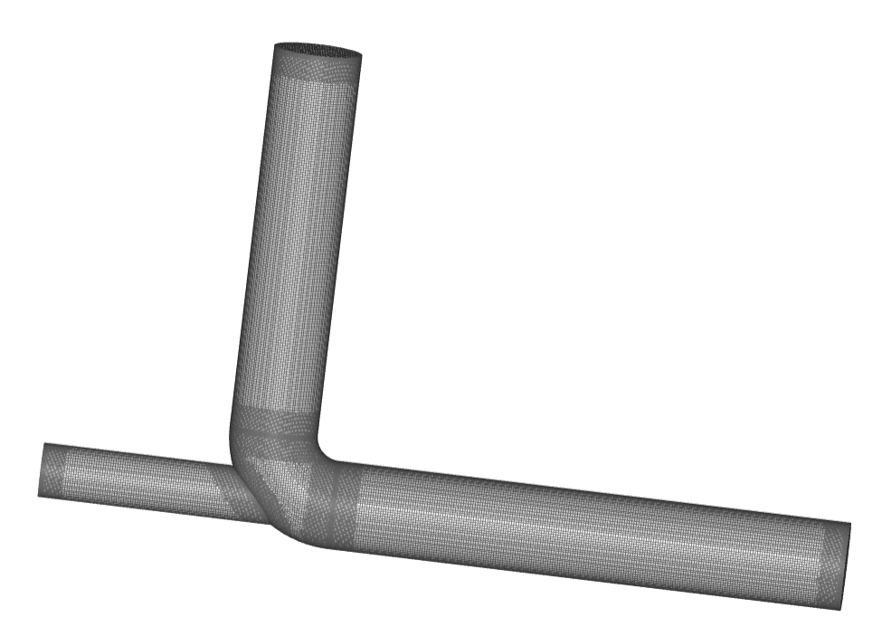
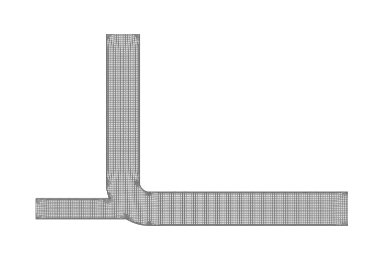
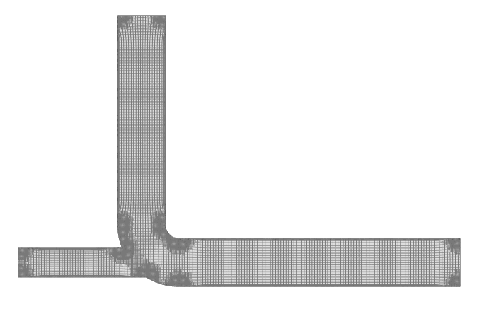
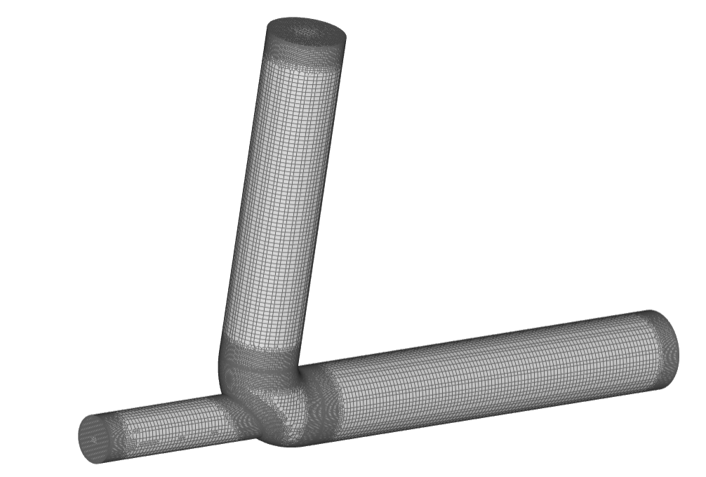
The finer mesh with feature refinement will be created after some minutes and look like Figure 23:
3.5. Mesh Five: Adding Surface Refinements
A surface refinement can be applied to refine cells on specific surfaces of the geometry. Both geometry faces and/or volumes can be selected for refinement. If a volume has been assigned, the refinement is applied to all surfaces of that volume.
It’s required to specify two refinement levels, the Minimum cell edge length, and the Maximum cell edge length. In a first step, a refinement up to the maximum length is applied across all of the assigned surfaces. Further refinement up to the minimum cell edge length is only applied to cells in areas where the normals form an angle greater than 30°. Therefore, in the following cases, only the first refinement step is applied:
- A flat surface
- A surface that has an angle between normals less than 30°
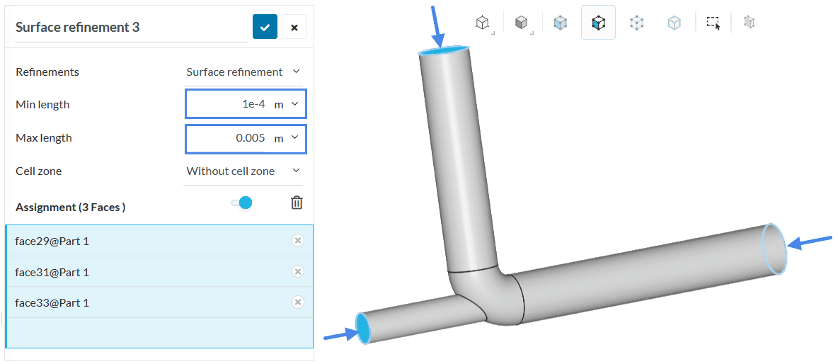
Copy the mesh settings from Mesh Four, and then choose the ‘Surface refinement‘. Before the Surface refinement is added, the pipe looks like this:
- Set the ‘Min length‘ to 0.0001 \(m\) and the ‘Max length‘ to 0.005 \(m\)
- Make sure the Assignment is toggled on.
- Apply the refinement on the three inlet and outlet faces.
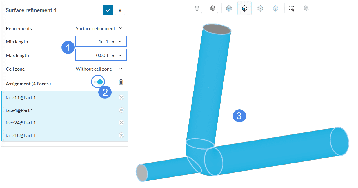
Proceed to create another surface refinement, this time for the rest of the faces of the pipe:
- Set the ‘Min length‘ to 0.0001 \(m\) and the ‘Max length‘ to 0.008 \(m\)
- Make sure the Assignment is toggled on.
- Select the four remaining faces of the pipe manually on the workbench.
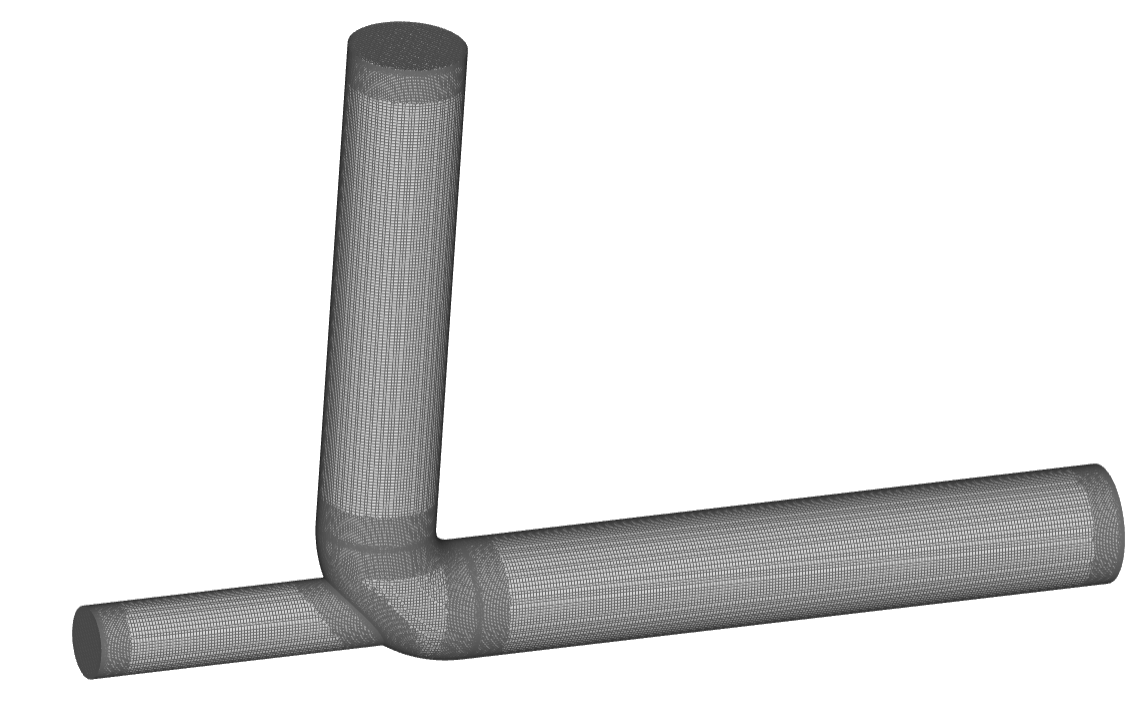
The final mesh takes less than one hour to run and has the following appearance.
4. Results
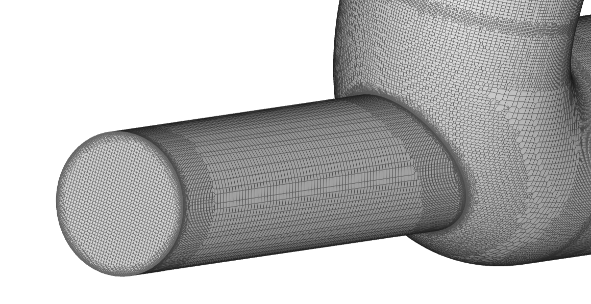
The boundary layer generation can easily be seen by zooming in on the mesh inlet.
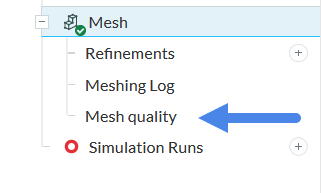
You can check the quality of your mesh and improve it by clicking on the ‘Mesh Quality‘ on the simulation tree. Use this article to help you examine the characteristics of your mesh.
Analyze your results with the SimScale post-processor. Have a look at our post-processing guide to learn how to use the post-processor.
Congratulations! You finished the tutorial!
Note
If you have questions or suggestions, please reach out either via the forum or contact us directly.
Last updated: December 23rd, 2025
Did this article solve your issue?
How can we do better?
We appreciate and value your feedback.


