Documentation
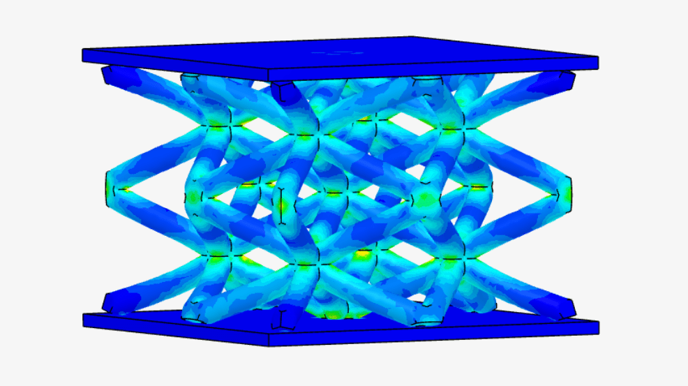
The Nonlinear Mechanical (Marc) analysis type is used to simulate intricate mechanical responses in structural elements and components subjected to significant deformation, challenging contact interactions—including self-contact—and strongly nonlinear material behaviors.
This analysis type is particularly well-suited for scenarios like metal forming, rubber part simulation, and the design of mechanical joints, where conventional linear approaches fall short.
Nonlinear Mechanical (Marc) is powered by ‘Marc™’. Marc™ is a registered trademark of HEXAGON.
Within SimScale, one can effortlessly set up a nonlinear mechanical simulation using the steps described below.
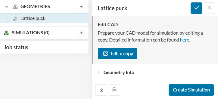
To create a Nonlinear Mechanical (Marc) analysis, first, select the desired geometry and click on ‘Create Simulation’:
Next, a window with a list of several analysis types supported in SimScale will be displayed:
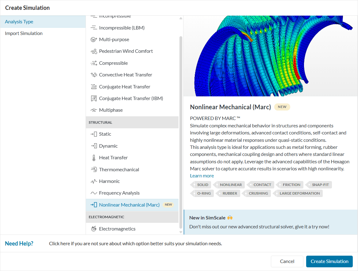
Choose the ‘Nonlinear Mechanical (Marc)’ analysis type and click on ‘Create Simulation’. This will lead to the Workbench with the following simulation tree and the respective settings:
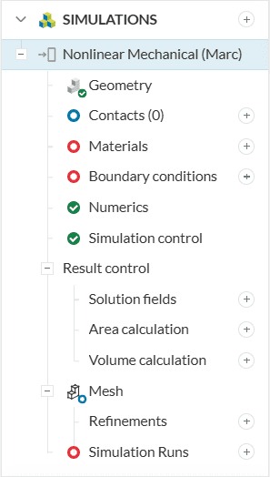
The Geometry section allows you to view and select the CAD model required for the simulation. It is important that the CAD model is well prepared to avoid any meshing or simulation-related errors. Find more details on CAD preparation and upload here.
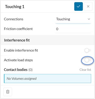
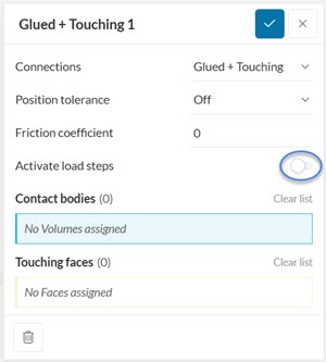
Here the user defines the contact interactions if the CAD is an assembly of multiple bodies. Glued, Touching, and Glued + Touching contact definitions are available. For more information about contacts, check this page.
To define the material properties of the domain, make sure to assign exactly one material to every part. Furthermore, you can choose the material behavior describing the constitutive law that is used for the stress-strain relation and the density of the material. Please see the materials section for more details.
Boundary conditions help to add closure to the problem at hand by defining how a system interacts with the environment. The following boundary conditions are supported:
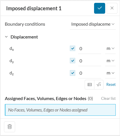
This is a boundary condition for the displacement vector variable. You can define prescribed values for the displacement of the assigned groups in every coordinate direction (x,y,z) or leave it unconstrained in order to let the entity move freely. Learn more.
In the Pressure boundary condition for structural simulations, a distributed load is applied on a face (or set of faces). It is useful to model the loads applied through the surface in contact with fluids or other solids, where the resultant of the load is in the normal direction of the face. Learn more.
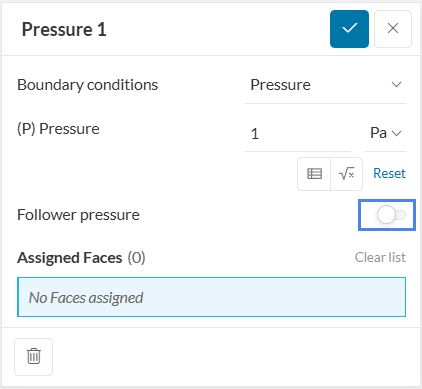
In contrast to the pressure boundary condition, the follower pressure is inherently nonlinear, as it will dynamically adapt during the simulation. Learn more.
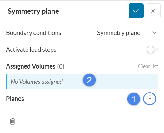
This boundary condition can be applied to enforce mirror-symmetry conditions on a structure, reducing the model’s size and computational time. This condition is imposed by creating planes (geometry primitives) and assigning those to the corresponding volumes which benefit from the symmetry condition.
With the Point Displacement boundary condition, it is possible to guide the displacement of an edge, face or volume through a remote point. This approach is suitable when the geometrical features connected to the point are expected to deform and/or have a prescribed rotation. With MARC, this boundary condition has the following settings:
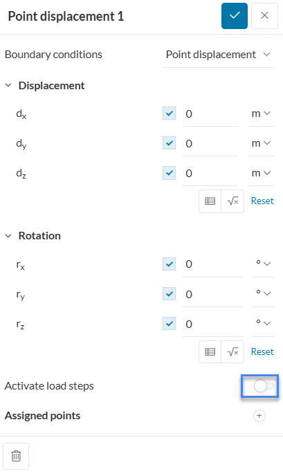
The parameters of the boundary conditions are:
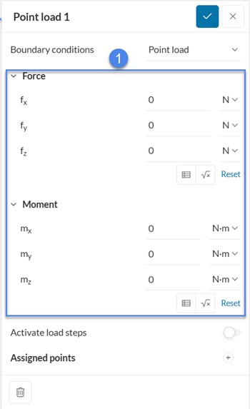
The Point Load boundary condition works similarly to the Remote Force boundary condition from our Static FEA module. In such case, the point load is applied to a remote point, which then is connected to an edge, face or volume with a rigid (RB2) or deformable (RB3) behavior. In the MARC solver, the definition of this condition is a three-step procedure. First, it is necessary to define values of forces and moments to be applied to a remote point:
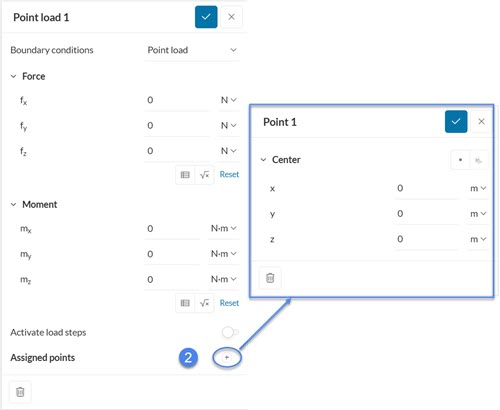
Second, the user needs to define the coodinates of the remote point:
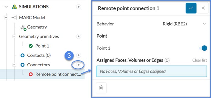
Third, the user needs to define a connector – this feature “connects” the point created to the corresponding edges, faces or volumes. Its behavior dictates if the assigned edges, faces or volumes are allowed to deform w.r.t to the point load applied.
Numerical settings play an important role in the simulation configuration. They define how to solve the equations by applying proper discretization schemes and solvers to the equations. They help enhance the stability and robustness of the simulation. Although all numerical settings are made available for users to have full control over, it is advised to keep them default unless necessary.
Numerical settings are recommended for advanced users but interested readers are encouraged to learn more about them through this documentation.
The Simulation control settings define the general controls over the simulation. In this tab, a series of variables can be set. For example, the End time and Maximum runtime for the simulation can be defined.
For a complete overview of the parameters and their meaning, check this page.
Under Result control, users can specify additional parameters of interest to be calculated. Monitors can also be defined. For example, one can set area and volume average controls, as well as point data for monitoring quantities on specific points. Additional solution fields such as displacement, strain, and contact result can be extracted too.
For more information about result controls, check this page.
Meshing is the process of discretization of the simulation domain. That means we split up a large domain into multiple smaller domains and solve equations for them. For a nonlinear mechanical analysis, the standard algorithm is available. For more information about meshes, make sure to check the dedicated page.
Last updated: January 30th, 2026
We appreciate and value your feedback.
Sign up for SimScale
and start simulating now