Solar Load

The electromagnetic radiation emitted by the sun is also referred to as solar radiation. In Computational Fluid Dynamics (CFD), solar radiation acts as an additional heat source. For some applications, such as thermal comfort studies, ignoring the solar radiation factor may impact the accuracy of the results.

In such cases, SimScale has a solar radiation module, available in the Conjugate Heat Transfer v2.0 analysis type, under the global settings, as shown in Figure 1:

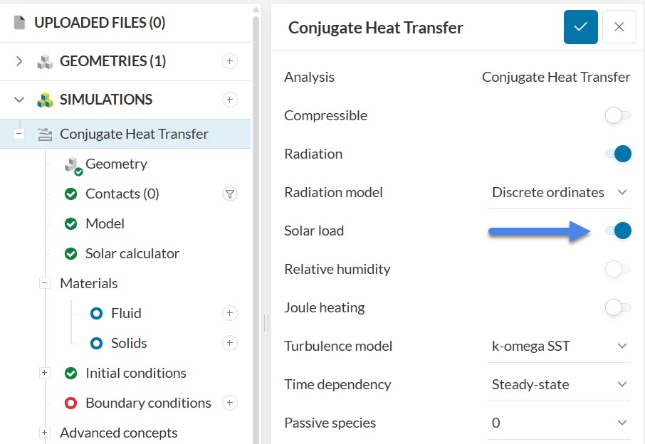
The solar radiation settings are found under Solar calculator in the simulation tree. Two main settings are required in the setup: the Sun direction, and the Solar load definitions. We will go through the details below.

Sun Direction

Under sun direction, the user can determine the position of the sun for their simulation. This is important because the direction of the solar rays changes based on the position of the sun.

In the Workbench, a set of yellow arrows will indicate the current direction of the sun rays, based on the Sun direction configuration. There are two options available for this setting: Time and place and Custom.

Time and Place

This configuration determines the position of the sun relative to the geometry for a given date, time, and location. It is worth mentioning that the sky is assumed to be in the positive z-direction, and the north direction is assumed to be in the positive y-direction. In case your model has a different orientation for the north direction, you can adjust the North angle in the settings.

Figure 3 shows the Time and place configuration steps:

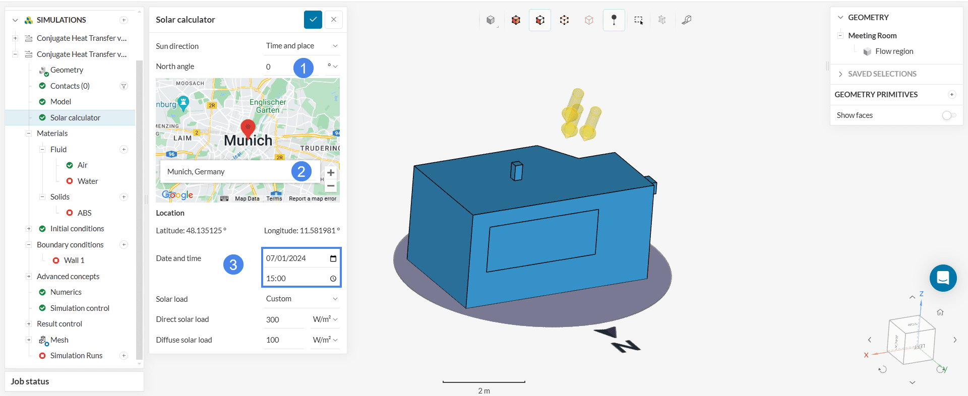
1. If the north direction is not positive y in your model, you can adjust the North angle.
2. In the interactive map, type the location where the model that you are simulating is located.
3. Choose a Date and time of interest.

SimScale will calculate the position of the sun relative to your model, given the date, time, and location.

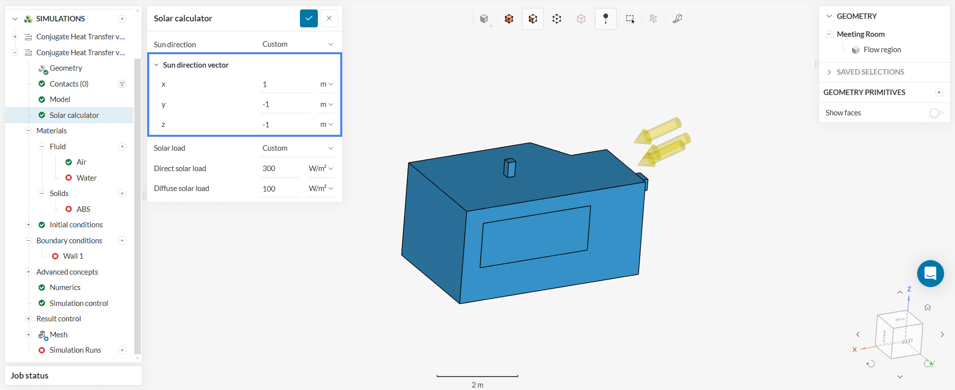
Custom

The second option is a custom definition of the Sun direction vector. Based on the orientation cube at the bottom-right of the Workbench, the user can define the direction of the sun’s rays:

Solar Load

After setting up the sun direction, we can define the Direct and the Diffuse solar loads that will be considered. Please check the next section in this documentation to see how different boundary conditions react to the solar load.

When an external opaque boundary of the model is exposed to either direct or diffuse radiation, the rays will act as a heat source to the boundary. With that being said, both direct and diffuse solar loads are considered external when they are absorbed by the external boundaries of the computational domain.

Furthermore, a direct solar load can also be absorbed by internal boundaries – This happens when a ray enters the domain via a transparent or semi-transparent boundary and hits an opaque boundary before exiting through another transparent or semi-transparent boundary. In this case, the solar load is internal.

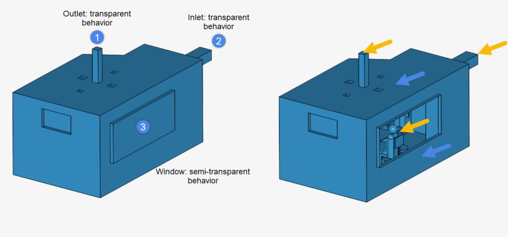
For example, let’s consider a meeting room with 3 transparent/semi-transparent boundaries, shown in the left-hand side room from Figure 5. In this case, the yellow arrows on the right-hand side room represent the internal solar load, while the blue arrows represent the external solar load.

Find below the two supported configurations for a solar load.

Custom

With a Custom definition for the solar load, the user can explicitly define the direct and diffuse solar load:

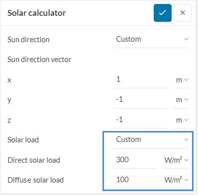
This option is useful in case you are interested in a specific value for the solar load.

Fair Weather Conditions

The Fair Weather Conditions method is an alternative way to define the diffuse and direct solar loads. For the underlying equations, please visit Table 14 from Chapter 29 in the 2001 ASHRAE Fundamentals Handbook\(^{[1]}\).

This approach assumes that the sky is in the positive z-direction, and the positive y-direction points to the north. For this reason, if you are using a Custom sun direction, the Sun direction vector must be negative in z. Otherwise, the sun would be below the horizon.

For the fair weather method, the user needs to provide a series of parameters, as shown below:

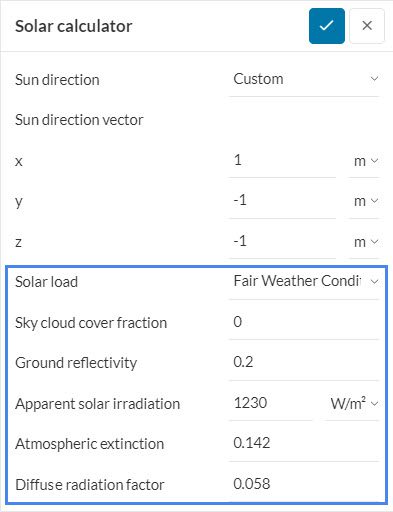
• The Sky cloud cover fraction represents the fraction of the sky which is taken by clouds.
• The Ground reflectivity depends on the color and texture of the ground around the computational domain.
• The remaining terms are related to extraterrestrial solar irradiance. Find below an adaptation of table 7, Chapter 30, from the 2001 ASHRAE Fundamentals Handbook\(^{[1]}\):

	Apparent Solar Irradiation \([\frac{W}{m²}]\)	Atmospheric Extinction	Diffuse Radiation Factor
January	1230	0.142	0.058
February	1215	0.144	0.060
March	1186	0.156	0.071
April	1136	0.180	0.097
May	1104	0.196	0.121
June	1088	0.205	0.134
July	1085	0.207	0.136
August	1107	0.201	0.122
September	1151	0.177	0.092
October	1192	0.160	0.073
November	1221	0.149	0.063
December	1233	0.142	0.057

Interactions with Boundary Conditions

The coupling of the solar load with the temperature field of the domain is done via boundary conditions. Once a boundary is hit by a ray, it will either absorb or transmit a fraction, or all of the incoming solar load. All boundary conditions transmit solar load in the same way, however, depending on their Temperature type definition, boundary conditions react differently to solar loads absorbed internally and externally.

Furthermore, under Solar radiative behavior, we define if a boundary is Transparent, Semi-transparent, or Opaque. Typically, inlets and outlets are transparent, whereas boundaries that do not allow light to travel through them are opaque. Certain materials, such as glass, are semi-transparent since they allow some light through.

Below, we are going to expand on the different Temperature type settings for a wall boundary condition.

Fixed Temperature

Since the boundary has a fixed temperature, the solar load does not have any effect.

Adiabatic

For internally absorbed solar load, the adiabatic boundary condition becomes a fixed gradient, forcing the wall to transfer heat to the adjacent fluid cells.

In the event of external solar load, the adiabatic configuration of the boundary prevents any external heat flux from entering the computational domain. Therefore, the external rays are completely blocked.

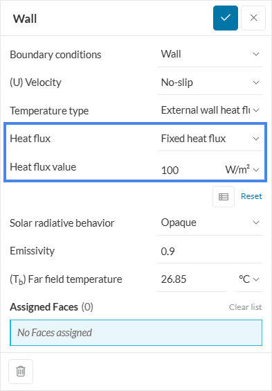
External Wall Heat Flux

When selecting External wall heat flux the user needs to define the Heat flux type, as seen in Figure 8. There are three options available:

1. Fixed heat flux: Since we define the fixed heat flux, we do not take any external solar load into account. However, the internal solar load is added to the fixed heat flux, resulting in more heat being dissipated to the adjacent flow region cells.
2. Fixed power: The behavior is the same as fixed heat flux. The external solar load does not affect this boundary condition, whereas internal solar loads will be added as a heat flux based on the surface area of the boundary.
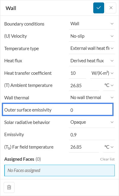
3. Derived heat flux: Both internal and external solar loads have an impact when using this configuration. The heat flux through this boundary is defined by the Heat transfer coefficient, the temperature differences, and the solar loads.

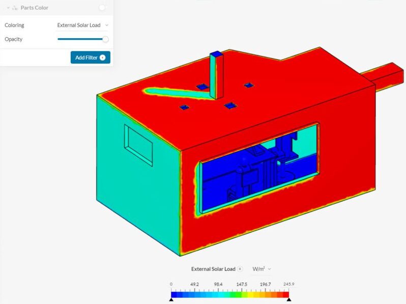
Post-processing

When simulating solar loads, it is possible to obtain the internal and external loads in the post-processor. For example, using the solar load settings from Figure 4, we have the following results:

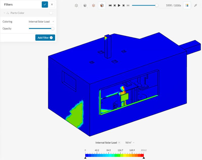
Now, inspecting the internal solar load, only the rays that go through the window (semi-transparent material) and the inlet/outlet (transparent) are taken into account.

It’s also possible to evaluate the thermal comfort parameters, such as PMV and PPD. For more details, please visit this documentation page.

Last updated: July 11th, 2023