When analyzing a structural system or other solid parts, it is often required to consider multiple load cases to model different operative scenarios. As it is often the case that users perform multiple separate simulations to solve for the different scenarios, in this article we will learn a workflow to unify all load cases into one simulation, and solve them in only one run.
Setting up the Loads
The first step in preparing our linear static simulation is to input the magnitude of the loads for each case. This is done by using the table input in the boundary condition setup panel, as shown for this example of an earthquake load, implemented as a Volume load:
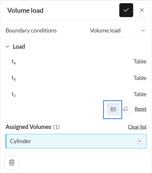
Click the ‘Table’ icon as highlighted in Figure 1 to open the table panel for the volume load. In the window that opens, we can input the various values for the load:
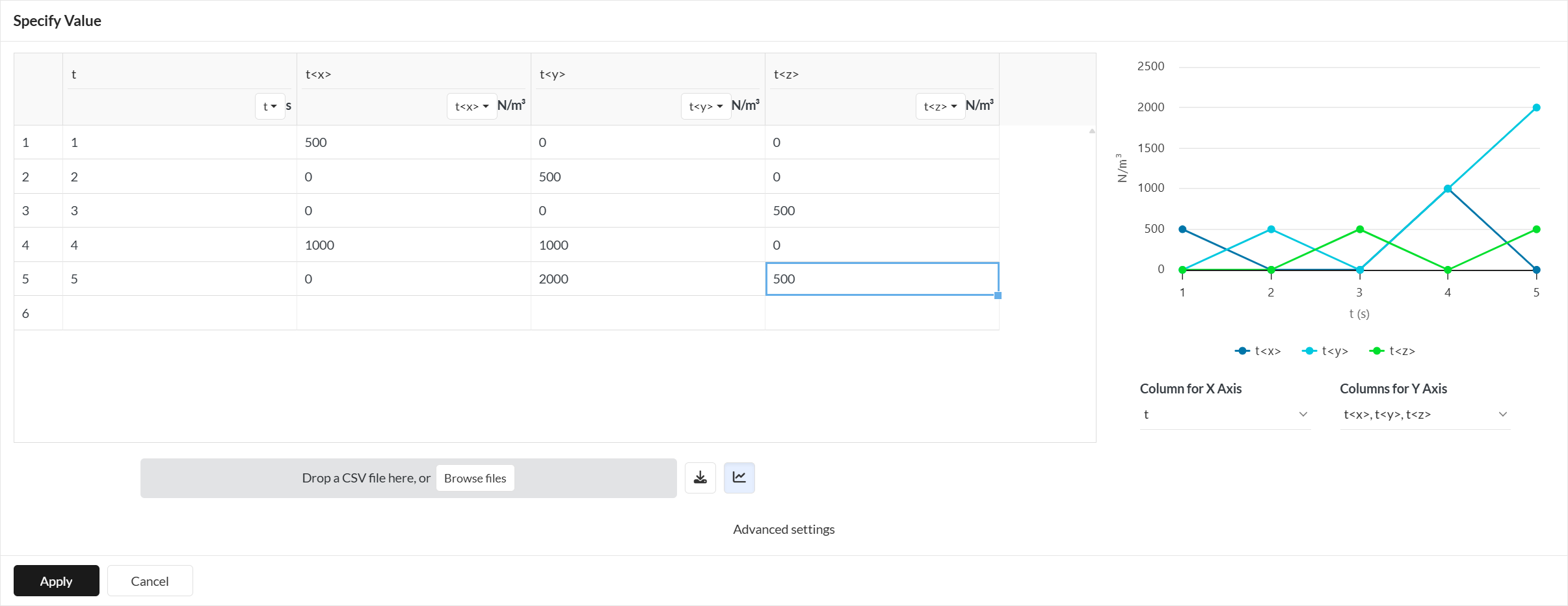
Notice how we have labeled each load case with the time variable and specified the value for the load components for each one of them, including the zero values when the load doesn’t apply. As we are performing a linear static simulation, the solution is independent of time. Thus, we can use the time variable to enumerate our load cases.
This typical setup should be applied to each one of the loads that vary across the cases. If one load is constant across all of them, the table input can be skipped for it.
Simulation Control
The next action is to specify the load cases, in terms of our ‘time’ variable, to be solved in the simulation run. This is done inside the Simulation control tab:
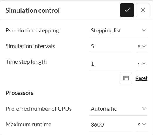
Notice the relevant setup:
- Pseudo time stepping is set to Stepping list,
- Simulation intervals is set to 9, to match the number of load cases in our example (see Figure 2),
- Time step length is set to 1, to make the pseudo time increment in integer values.
This is enough information for the solver to compute and save the solution at all of our load cases.
Post-Processing
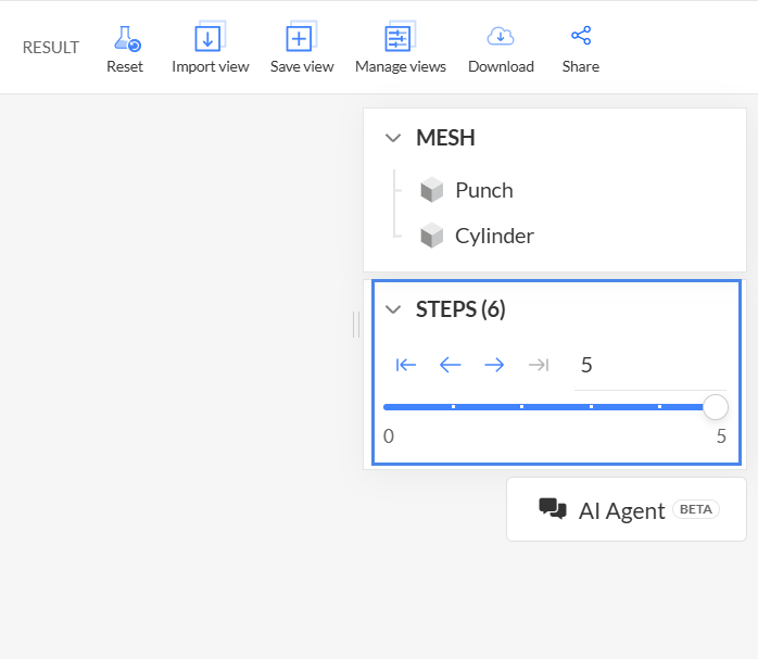
When the simulation run is complete, we can go to the online post-processor, where we can navigate through the load cases using the frame (time) selection toolbox at the top:
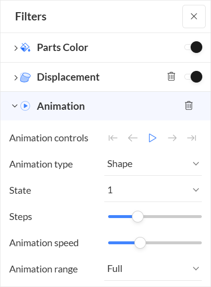
If we want to animate the results at a given load case, then we must change the Animation type to Shape, and select the load case number in the State field:
This concludes our presentation of the workflow. For more information about finite element analysis, be sure to check out the following tutorials:


