How to Predict Linear and Exponent Coefficients for a Power Law Porous Media?

In this article, you will learn how to predict linear and exponent coefficients for a power law porous media modeling using experimental data.

Overview

In our simulations, often times we have to model a structure as a porous media. These structures can be as simple as perforated plates and as complex as radiators. The objective, however, is the same: save mesh cells while still accounting for local pressure losses.

In the Power Law formulation, pressure losses are given by:

$$\Delta P = C_0 \cdot \rho \cdot L \cdot U^{C_1}$$

where:

• \(\Delta P\) is the pressure drop across the porous media \([Pa]\);
• \(\rho\) is the density of the fluid \([kg/m³]\);
• \(L\) is the thickness of the porous zone \([m]\);
• \(U\) is the fluid velocity \([m/s]\);
• \(C_0\) is the linear coefficient and;
• \(C_1\) is the exponent coefficient.

Power Curve Fitting Approach

Using experimental data for pressure versus velocity, we can extract the coefficients.

For example, let’s take a 0.01 meters thick perforated plate and water as fluid. The following case was simulated in SimScale at 6 different velocities.

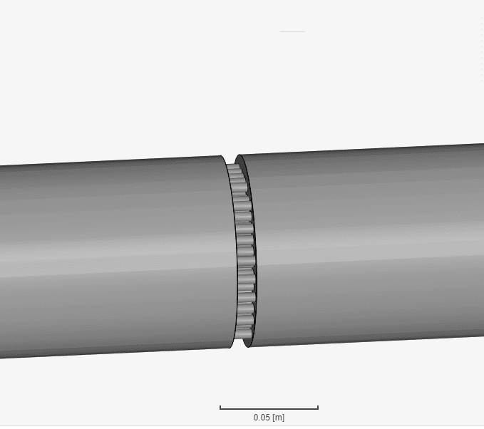
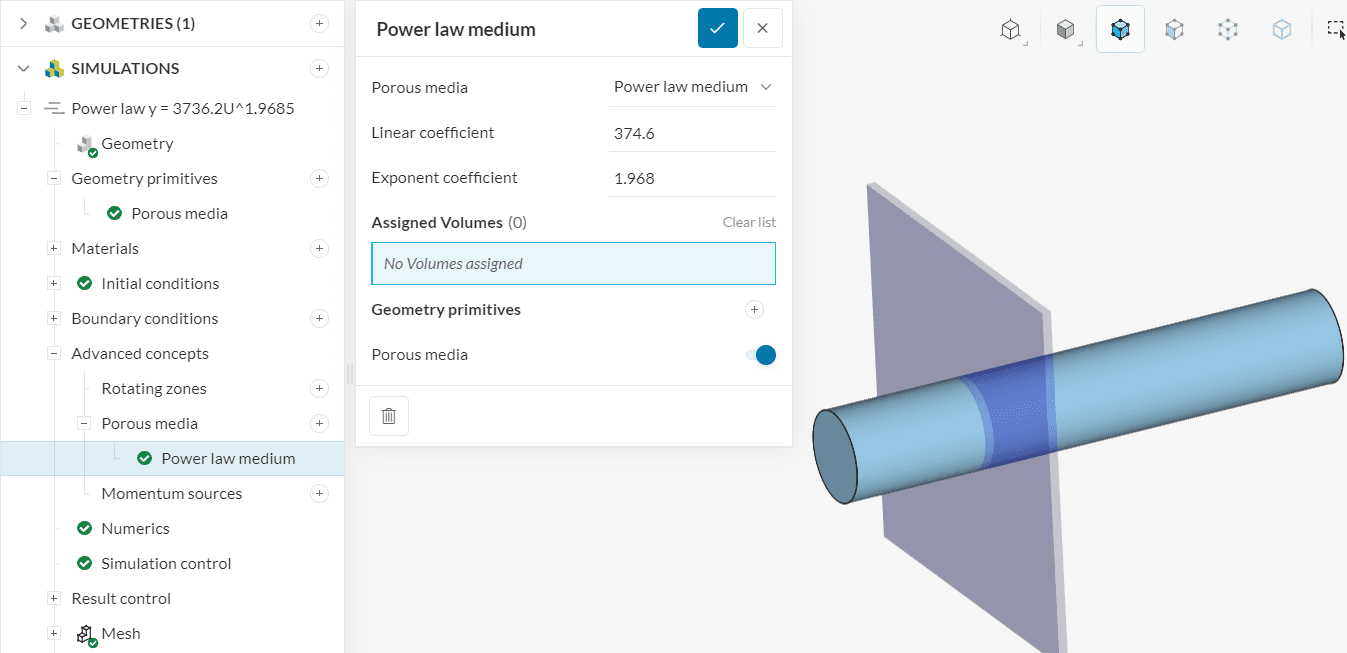
Instead of simulating the original geometry of the perforated plate, we will model it as a porous medium. In the platform, you can readily create a porous media and assign it to a volume or a geometry primitive such as the cartesian box shown below:

The table below shows the results from the simulations:

Velocity \([m/s]\)	Pressure drop \([Pa]\)
0.5	960
0.7	1840
1	3720
1.2	5390
1.5	8240
2	14690

By fitting this data set with a power curve, we get the following:

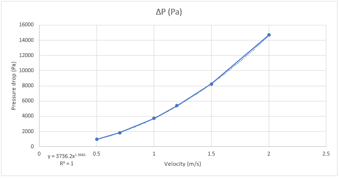
The expression below is extracted from the plot:

$$\Delta P = 3736.2 \cdot U^{1.9685}$$

From that, we obtain \(C_0\) and \(C_1\):

$$C_0 = {3736.2 \over \rho \cdot L} = {3736.2 \over 997.33 \cdot 0.01} = 374.62$$

$$C_1 = 1.9685$$

Now to compare experimental data with simulation results:

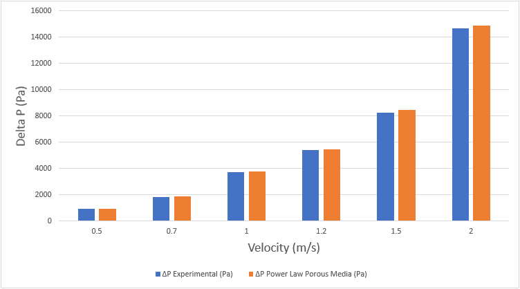
Thus, the power law model proves to be accurate in accounting for pressure losses.