Validation Case: Thermal Comfort in Room with Underfloor Air Distribution
The underfloor air distribution validation case belongs to fluid and thermodynamics. This case aims to validate the correct calculation of temperature and air speed distributions in a mechanically ventilated room.
The validation is performed against experimental data obtained by Zhang and Chen\(^1\), who analyzed the particle transport and distribution in ventilated rooms.
It is possible to use their results because it was concluded that those particles were passive scalars and, therefore, had no impact on the fluid behavior or the room temperature.
Geometry
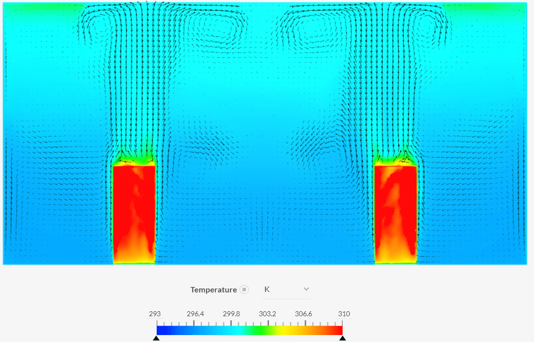
The geometry consists of a room with an underfloor air distribution (UFAD) ventilation system. The heat sources used are four human simulators and six ceiling lights.
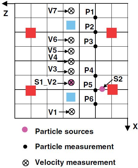
Cool air is fed to the room through the inlets on the floor, while the humans and the lamps heat the surrounding air, creating convection currents. Figure 1 gives an overview of the geometry and room dimensions.
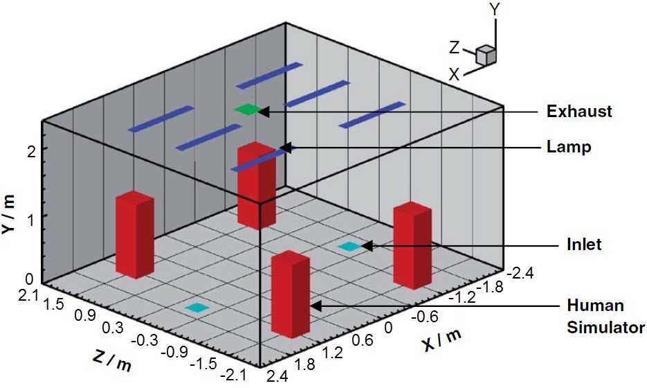
Although the figure adapted from Zhang and Chen\(^1\) has a scale; the only details provided by the paper were the dimensions of the room. Based on that and other schematic figures provided in the reference paper, it was possible to estimate closely the dimensions of the other elements.
The geometry used in the present air distribution validation case is shown below:
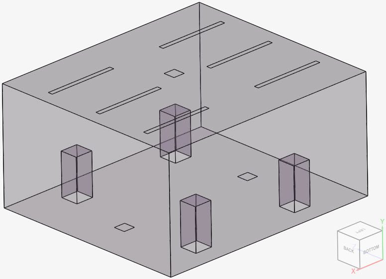
Table 1 gives further details on the dimensions of each element:
| Element | Length in x-Direction \([m]\) | Length in y-Direction \([m]\) | Length in z-Direction \([m]\) |
| Room | 4.8 | 4.2 | 2.4 |
| Human Simulator | 0.38 | 0.9 | 0.38 |
| Inlets | 0.25 | – | 0.25 |
| Exhaust | 0.25 | – | 0.25 |
| Lamps | 1.5 | – | 0.1 |
Analysis Type and Mesh
Tool Type: OpenFOAM®
Analysis Type: Steady state, incompressible convective heat transfer analysis
Turbulence Model: k-epsilon
Mesh and Element Types: The mesh used in this validation case was created in SimScale with the standard algorithm. Appropriate refinements on the lamps, human simulators, inlets, and exhaust surfaces were applied. Additionally, boundary layer refinements were applied on all surfaces, to ensure the correct results of the thermal boundary layer.
Table 2 presents metrics and details of the resulting mesh:
| Domain | Mesh Type | Cells | Element Type |
| Room | Standard | 3340621 | 3D tetrahedral/hexahedral |
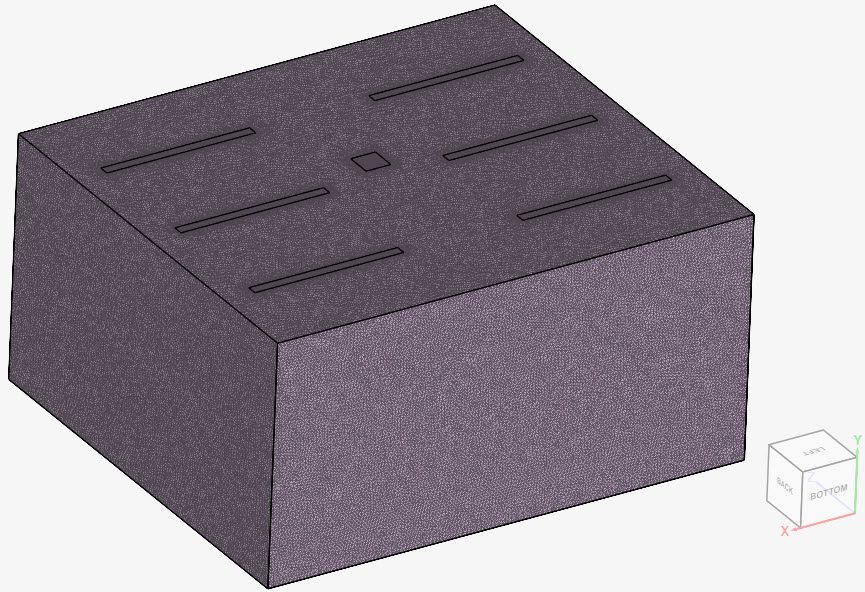
Find below, in Figure 3, the standard mesh generated in SimScale.
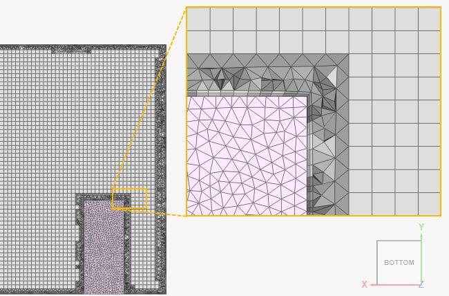
Using a mesh clip to inspect the interior cells, it’s possible to observe the transition from tetrahedral cells to hexahedral cells. The boundary layers are also visible:
Simulation Setup for Underfloor Air Distribution
In the reference paper, the authors provided the power generation for the human simulators as a whole. For the air distribution simulation, the total power was distributed according to each face of the simulators. Additionally, the Boussinesq approximation (incompressible flow) was used for this simulation as no significant temperature differences would be present.
Material:
- Viscosity model: Newtonian
- \((\nu)\) Kinematic viscosity: 1.5295e-5 \(m^2/s\)
- \((\rho)\) Density: 1.1965 \(kg/m^3\)
- Thermal expansion coefficient: 0.00343 \(\frac {1} {K}\)
- \((T_0)\) Reference temperature: 298.15 \(K\)
- \((Pr_{lam})\) Laminar Prandtl number: 0.713
- \((Pr_{t})\) Turb. Prandtl number: 0.85
- Specific heat: 1004 \(\frac {J} {kg.K}\)
Boundary Conditions:
The boundary conditions will be defined based on the nomenclature and orientation of Figure 1.
In the table below, the configuration for both velocity and pressure are given at each of the boundaries:
| Element | Boundary Type | Boundary Condition Description |
| Inlet | Velocity inlet | 0.0472 \(m^3/s\) per inlet, at 293 \(K\) |
| Exhaust | Pressure outlet | Gauge pressure fixed at 0 \(Pa\) |
| Human simulators (top face) | Wall | No-slip condition with a turbulent heat flux. The power heat source is defined as 9.6 \(W\) per face. |
| Human simulators (side faces) | Wall | No-slip condition with a turbulent heat flux. The power heat source is defined as 22.6 \(W\) per face. |
| Lamps | Wall | No-slip condition with a turbulent heat flux. The power heat source is defined as 64 \(W\) per lamp. |
| Wall: positive x-direction | Wall | No-slip condition, with a fixed temperature of 297.7 \(K\) |
| Wall: negative x-direction | Wall | No-slip condition, with a fixed temperature of 298 \(K\) |
| Ceiling: positive y-direction | Wall | No-slip condition, with a fixed temperature of 298.7 \(K\) |
| Floor: negative y-direction | Wall | No-slip condition, with a fixed temperature of 297 \(K\) |
| Wall: positive z-direction | Wall | No-slip condition, with a fixed temperature of 298.5 \(K\) |
| Wall: negative z-direction | Wall | No-slip condition, with a fixed temperature of 298.3 \(K\) |
Numerics
The following settings are different from the default:
- Relaxation type: Manual
- \((P)\) Modified pressure field: 0.7
- \((U)\) Velocity equation: 0.3
- \((T)\) Temperature equation: 0.5
- \((k)\) Turb. kinetic energy equation: 0.7
- \((\epsilon)\) Dissipation rate equation: 0.7
- Divergence scheme
- div(phi,U): Gauss linear upwind limited grad
Result Comparison
In the reference study, the authors evaluated seven lines with probe points across the middle of the room \((z = 0)\). Each line contains up to 7 probe points, located at \(y\) = {0.1, 0.3, 0.6 1.1, 1.4, 1.7, 2.2} meters.
The location of the probe points was obtained from Figure 5, provided in the reference paper:
Velocity Profiles
The lines of interest for this validation case were V1, V2, and V3. Find the comparison between the reference study and the SimScale results for velocity in Figure 6:
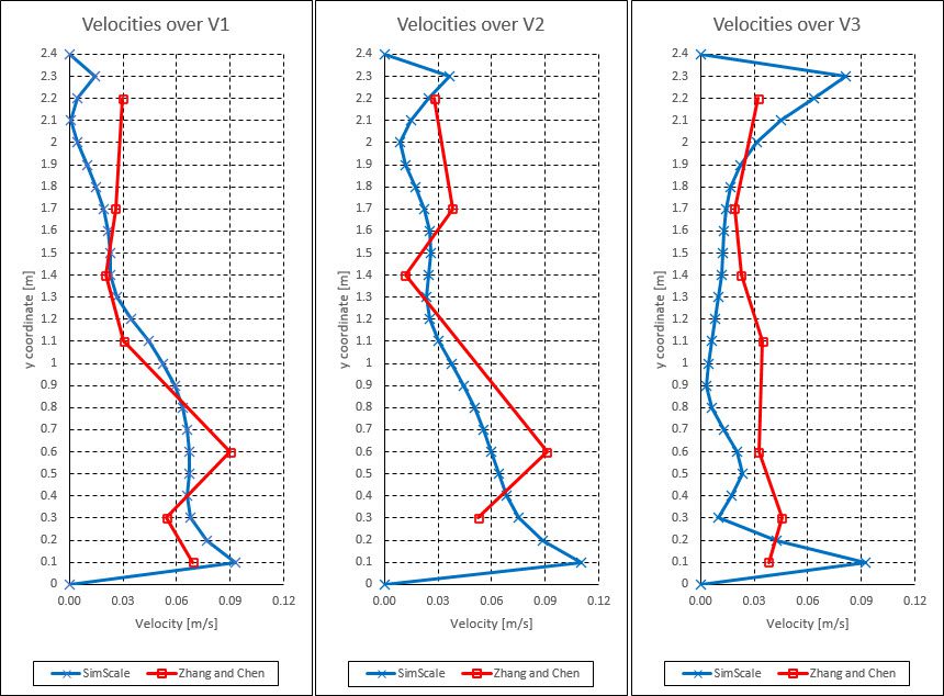
A comparison of the velocity profiles reveals that the SimScale results follow the same trend as the experimental results provided by the reference\(^1\). Since many dimensions had to be estimated and tested, discrepancies were expected.
Additionally, the results provided by Zhang and Chen lack symmetry across the ZY plane, which should not be the case given that the geometry is symmetric. These errors in the experimental results add to the discrepancies between SimScale and the reference values. The most important thing is that the profiles follow the same trend.
Temperature Profiles
A similar comparison was done for temperatures. The temperatures were normalized using equation 1:
$$T_{norm} = \frac {T-T_{inlet}} {T_{exhaust}-T_{inlet}}\tag{1}$$
In SimScale’s results, \(T_{exhaust}\) was found to be 299.15 \(K\). In Figure 7, we compare the simulation results to values from the reference paper.
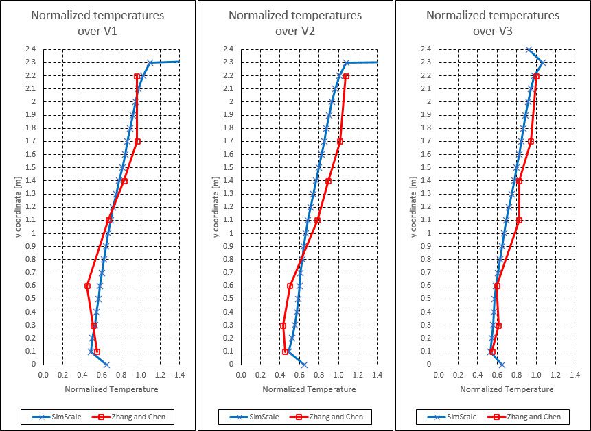
A comparison of the temperature profiles reveals that the SimScale results follow the same trend as the experimental results, even more closely than the velocity ones. As explained above, disparities were to be expected.
Having such close results for the temperature indicates that the difference in the velocity profile comes from the estimated size of the inlet sizes, which impacts velocity and not temperature.
Last updated: March 28th, 2025
Did this article solve your issue?
How can we do better?
We appreciate and value your feedback.


