Validation Case: Thermal Bridge Case 4 – Iron Bar

This thermal bridge validation case belongs to heat transfer. The aim of this test case is to validate the following parameters:

• Temperature distribution
• Heat flow

The simulation results of SimScale were compared to the results presented in EN ISO 10211 Standard, case 4.

Geometry

The 3D geometry for this project is a thermal bridge consisting of an iron bar penetrating an insulation layer, as seen in Figure 1:

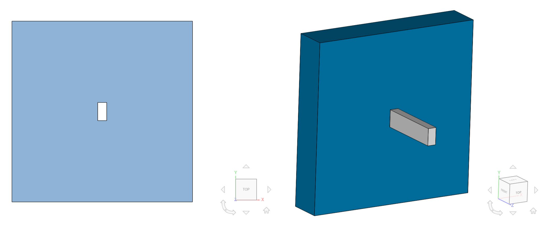
The insulated wall consists of a block with a rectangular cross-section of 1×1 \(m\) and a width of 0.2 \(m\). The bar is placed vertically in the center of the wall and goes through the whole layer. It has a rectangular cross-section of 0.1×0.05 \(m\) and a total length of 0.6 \(m\), including its penetrated part.

Analysis Type and Mesh

Tool Type: Code_Aster

Analysis Type: Linear, steady-state heat transfer analysis

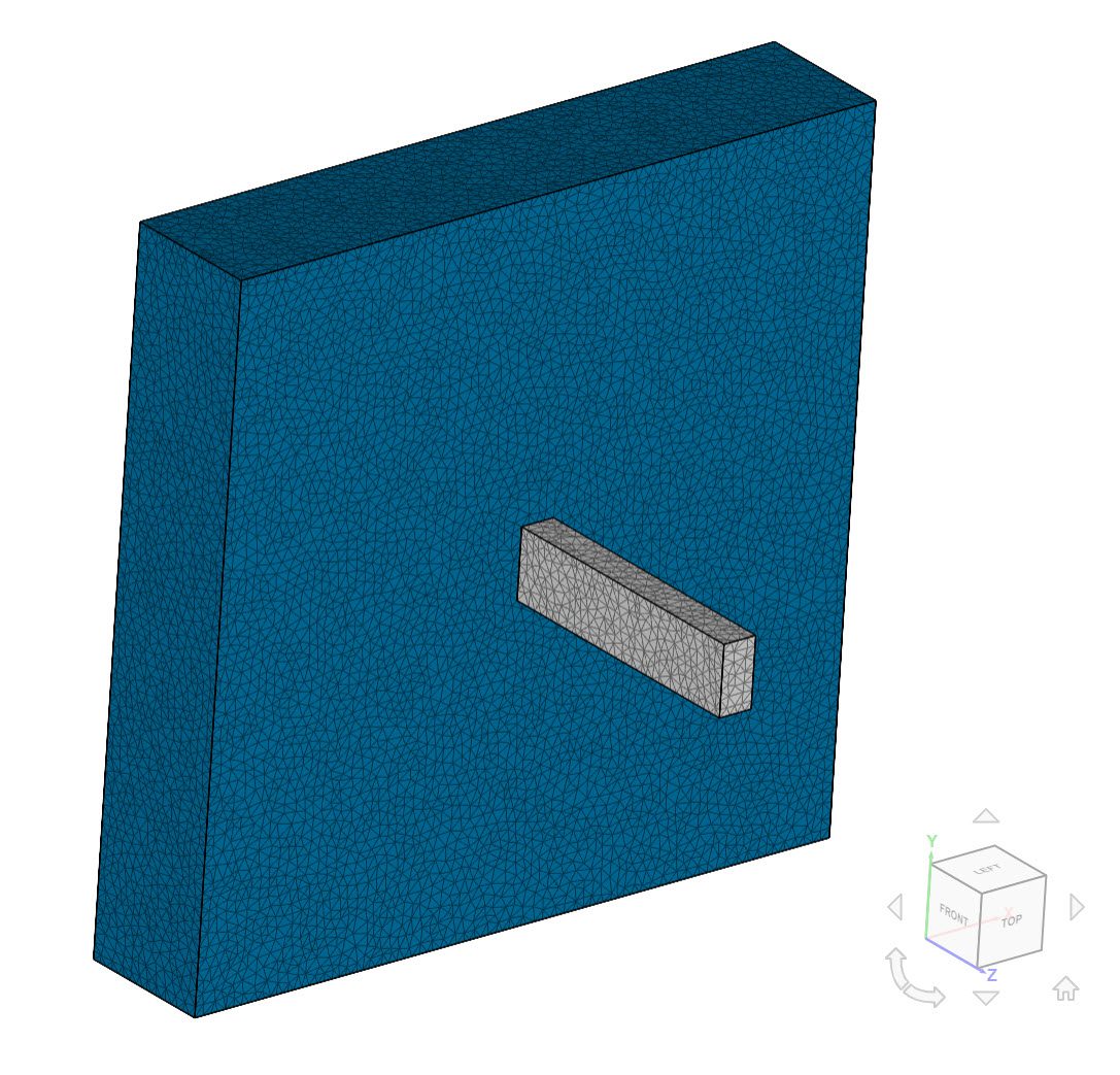
Mesh and Element Types: For this case, SimScale’s standard meshing algorithm was used, which generates a combination of tetrahedral and hexahedral cells. The characteristics of the resulting mesh can be seen below:

Case	Mesh Type	Nodes	Cells	Element Type
EN ISO 10211 Case 4	Second-order standard	769105	553835	Standard

In the image below, it’s possible to see the standard mesh in detail:

Simulation Setup

Material:
Each body is assigned to a different material:

• Insulation layer
  • (\(\rho\)) Density: 2240 \(\frac{kg}{m^3}\)
  • Thermal conductivity: 0.1 \(\frac{W}{m.K}\)
  • Specific heat: 750 \(\frac{J}{kg.K}\)
• Iron bar
  • (\(\rho\)) Density: 7870 \(\frac{kg}{m^3}\)
  • Thermal conductivity: 50 \(\frac{W}{m.K}\)
  • Specific heat: 480 \(\frac{J}{kg.K}\)

Boundary Conditions:

As shown in Figure, the following boundary conditions are defined:

• Interior wall: Convective heat flux boundary condition:
  • (\(T_0\)) Reference temperature: 1 \(ºC\)
  • Heat transfer coefficient: 10 \(\frac{W}{m^2.K}\)
• Exterior wall: Convective heat flux boundary condition:
  • (\(T_0\)) Reference temperature: 0 \(ºC\)
  • Heat transfer coefficient: 10 \(\frac{W}{m^2.K}\)
• Side walls: Adiabatic in nature.

Result Comparison

The results obtained with SimScale were compared to those presented in [1]. The two criteria that must be satisfied are:

• The difference in heat flow between the hot and cold sides should not deviate more than 1 % from the reference value of 0.540 \(W\).

• The highest temperature measured in the exterior wall should not deviate more than 0.005 \(°C\) from the reference value of 0.805 \(°C\).

The bulk calculator feature provided in SimScale’s integrated post-processor was used to extract the maximum temperature of the beam’s end cross-section, which is coincident with the insulation layer. The Heat Flux was measured using the Heat Flow result control Item. The table below provides an overview of the results:

Result	Reference Value	SimScale Result	Deviation
Maximum temperature on exterior	0.805\(°C\)	0.803\(°C\)	0.002\(°C\)
Heat Flow	0.540\(W\)	0.542\(W\)	-0.37%

Table 4 indicates a good agreement of the SimScale results with the reference paper, with a permitted difference between the extracted values and the standard.

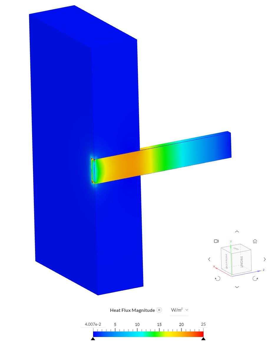
Below you can see the results of the simulation, created in the online post-processor:

Additionally, the heat flux magnitude can be visualized on the cutting plane normal to the X axis too:

Last updated: August 30th, 2022