Validation Case: Impact of an Elastoplastic Bar

This validation case belongs to an elastoplastic impact in solid mechanics. The aim of this test case is to validate the following parameters:

Dynamic analysis
Frictional contact
Elastoplasticity
Large deformations

The simulation results of SimScale were compared to the numerical results presented in [SDNV103]\(^1\).

View Project

Geometry

The geometry used for the case is as follows:

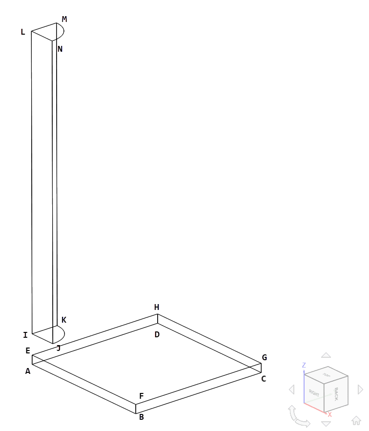
geometrical model for dynamic elastoplastic impact validation case — Figure 1: Geometrical model of the impact bar and plate

It represents an elastoplastic bar in the z-direction and a rectangular plate in the x-y plane with the following coordinates for each point:

Point	X [m]	Y [m]	Z [m]
A	0	0	0
B	0.016	0	0
C	0.016	0.016	0
D	0	0.016	0
E	0	0	0.001
F	0.016	0	0.001
G	0.016	0.016	0.001
H	0	0.016	0.001
I	0	0	0.00327
J	0.0032	0	0.00327
K	0	0.0032	0.00327
L	0	0	0.03567
M	0.0032	0	0.03567
N	0	0.0032	0.03567

Table 1: Coordinates of the geometry vertices

Analysis Type and Mesh

Tool Type: Code Aster

Analysis Type: Dynamic

Mesh and Element Types: The meshes used in this project were created in SimScale with the standard algorithm. Manual refinements are used to control the cell sizes.

Case	Element Type	Number of Nodes	Element Technology
A	1st Order Tetrahedral	10435	Standard
B	2nd Order Tetrahedral	70001	Reduced Integration

Table 2: Mesh details for each case.

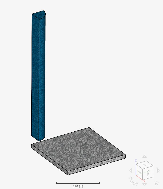
Find below the mesh used for case B. It’s a standard mesh with second-order tetrahedral cells.

hexahedral mesh for dynamic elastoplastic impact validation case — Figure 2: Finite elements mesh as used on case B

Simulation Setup

Material:

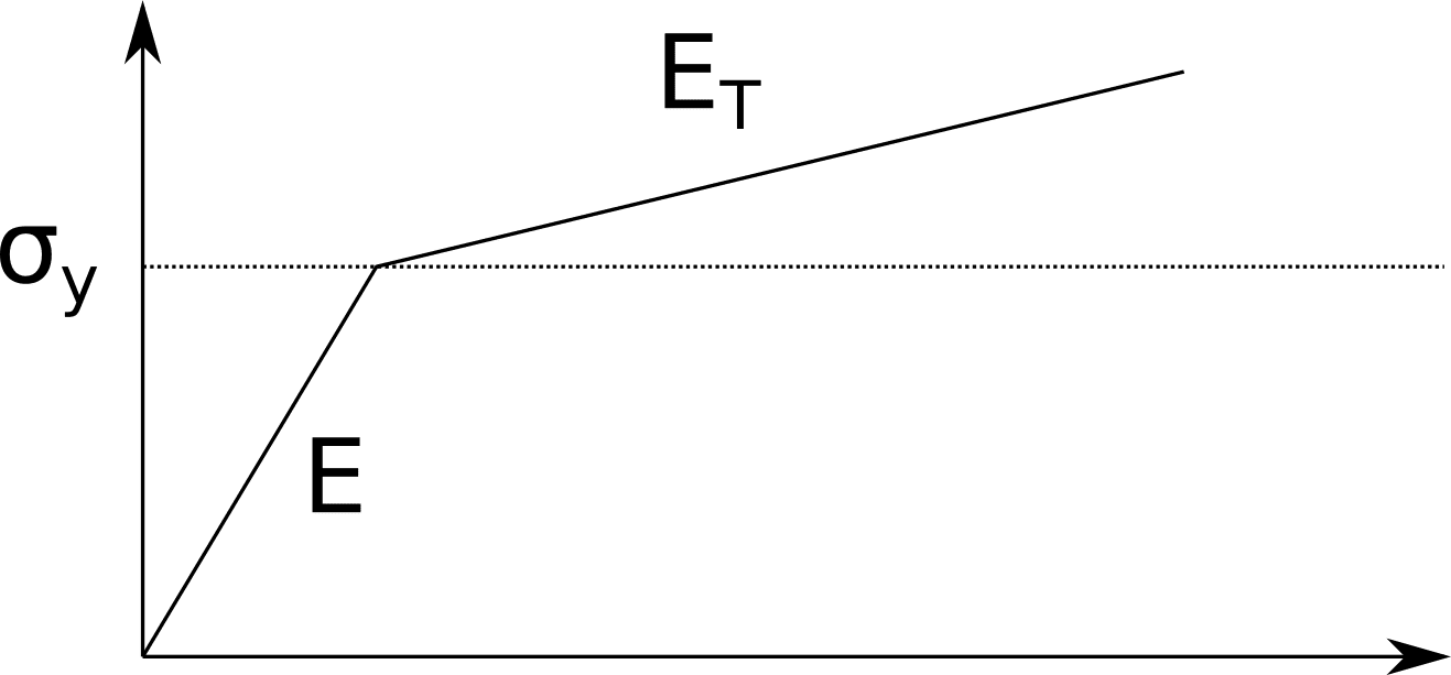
Bi-linear Plasticity Isotropic:
- \( E = \) 117 \( GPa \)
- \( \nu = \) 0.35
- \( \sigma_y = \) 400 \( MPa \)
- \( E_T = \) 500 \( MPa \)

Boundary Conditions:

Initial Conditions:
- Velocity of 227 \(m/s \) to volume IJKLM (bar)
Constraints:
- Volume ABCDEFGH (plate) fixed
- Face IKLN zero x-displacement
- Face IJLM zero y-displacement

Reference Solution

The reference solution is from a numerical computation as presented section 2 of [SDNV103]\(^1\), which are taken as the mean results of [Stainer]\(^2\):

\( DX_J = 3.87 mm \)

\( DZ_L = 13.46 mm \)

Result Comparison

Comparison of displacements at points J (DX) and L (DZ) at time \( t = 9×10^{-5}\ s \):

CASE	POINT	COMP	COMPUTED	REF	ERROR
A	J	DX	0.00289	0.00387	-25.4%
A	L	DZ	-0.01250	-0.01346	-7.1%
B	J	DX	0.00365	0.00387	-5.8%
B	L	DZ	-0.01265	-0.01346	-6.0%

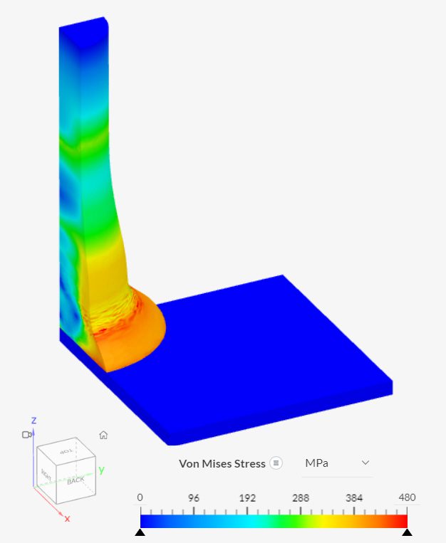
Table 3: Results comparison and computed error.

An illustration of the final shape (case B) can be found in Figure 4. The elastoplastic deformation due to the impact can be appreciated:

results plot for dynamic elastoplastic impact validation case — Figure 4: Deformed shape with stress plot at t = 9e-5 \(s\) from case B

Tutorial: Crash Test of FSAE Impact Attenuator

References

https://www.code-aster.org/V2/doc/default/en/man_v/v5/v5.03.103.pdf
Results by Stainier et al. as mentioned in [SDNV103]: L. Stainier and J.Ph. Ponthot. An improved one-point integration method for large strain elastoplastic analysis. Computer Methods in Applied Mechanics and Engineering, 118(1–2):163 – 177, 1994

Note

If you still encounter problems validating you simulation, then please post the issue on our forum or contact us.

Last updated: September 30th, 2021

Did this article solve your issue?

How can we do better?

We appreciate and value your feedback.