Validation Case: Heat Transfer in a Perforated Plate
This project belongs to the heat transfer analysis type. The aim of this test case is to validate the following parameter using a transient thermal solver, with a surface and a convective heat flux boundary condition on a perforated plate:
- Temperature \([K]\) on a single node for 12 consecutive timesteps.
The simulation results of SimScale were compared to the results presented in case B of [TTLP301]\(^1\).
Geometry
The geometry used for the analysis with the highlighted node N1 can be seen below. It is a random thick plate with straight and curved edges.
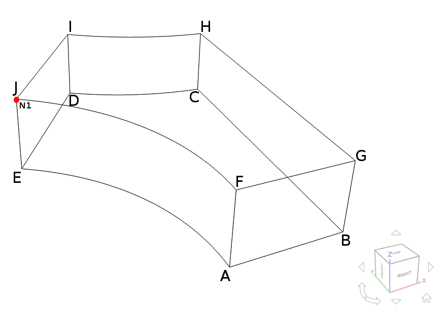
The coordinates for each vertex of the plate are displayed in the following table:
| A | B | C | D | E | F | G | H | I | J | |
|---|---|---|---|---|---|---|---|---|---|---|
| x \([m]\) | 0.635 | 0.9395 | 0.9395 | 0.5427 | 0.3175 | 0.635 | 0.9395 | 0.9395 | 0.5428 | 0.3175 |
| y \([m]\) | 0 | 0 | 0.8338 | 0.9401 | 0.5499 | 0 | 0 | 0.8338 | 0.9401 | 0.5499 |
| z \([m]\) | 0 | 0 | 0 | 0 | 0 | 0.2 | 0.2 | 0.2 | 0.2 | 0.2 |
Analysis Type and Domain
Tool type : Code_Aster
Analysis type : Heat transfer, linear
Time dependency: Transient
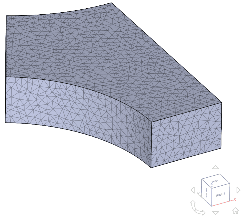
Mesh and element types: Two mesh cases were considered for the analysis of the perforated plate, with 1st order and 2nd order tetrahedral elements:
| Case | Mesh type | Number of nodes | Number of 3D elements | Element type |
|---|---|---|---|---|
| (A) | Standard | 5340 | 25676 | 1st order tetrahedral |
| (B) | Standard | 16807 | 10976 | 2nd order tetrahedral |
Below, the 1st order tetrahedral mesh for case A is visualized:
Simulation Setup
Material/Solid
- Isotropic:
- Density \(ρ\) = 1 \( kg \over \ m³ \),
- Thermal conductivity \(\kappa\) = 0.1 \( W \over \ m \ K\),
- Specific heat = 1 \( J \over \ kg \ K\)
Initial conditions
- Initial Temperature = 273.15 \(K\)
Boundary conditions
- Surface heat flux on face AFJE:
- Heat flux value = 1 \(W \over \ m²\)
- Convective heat flux on face CHID
- Reference temperature \(T_{0}\) = 273.15 \(K\)
- Heat transfer coefficient = 1 \(W \over \ m² \ K\)
Results Comparison
The temperature values at node N1 for 12 time steps obtained with SimScale are compared against the results presented in case B of [TTLP301]\(^1\).
| Timesteps \([s]\) | [TTLP301] \([K]\) | Case A \([K]\) | Error [%] | Case B \([K]\) | Error [%] |
|---|---|---|---|---|---|
| 0.1 | 274.195 | 274.201 | 2.19E-03 | 274.203 | 2.92E-03 |
| 0.2 | 274.597 | 274.601 | 1.46E-03 | 274.604 | 2.55E-03 |
| 0.3 | 274.892 | 274.895 | 1.09E-03 | 274.898 | 2.18E-03 |
| 0.4 | 275.132 | 275.135 | 1.09E-03 | 275.138 | 2.18E-03 |
| 0.5 | 275.339 | 275.342 | 1.09E-03 | 275.345 | 2.18E-03 |
| 0.6 | 275.523 | 275.526 | 1.09E-03 | 275.529 | 2.18E-03 |
| 0.7 | 275.691 | 275.695 | 1.45E-03 | 275.697 | 2.18E-03 |
| 0.8 | 275.848 | 275.852 | 1.45E-03 | 275.854 | 2.18E-03 |
| 0.9 | 276.996 | 275.999 | 1.09E-03 | 276.001 | 1.81E-03 |
| 1.0 | 276.136 | 276.14 | 1.45E-03 | 276.142 | 2.17E-03 |
| 1.1 | 276.27 | 276.274 | 1.45E-03 | 276.276 | 2.17E-03 |
| 1.2 | 276.398 | 276.403 | 1.81E-03 | 276.404 | 2.17E-03 |
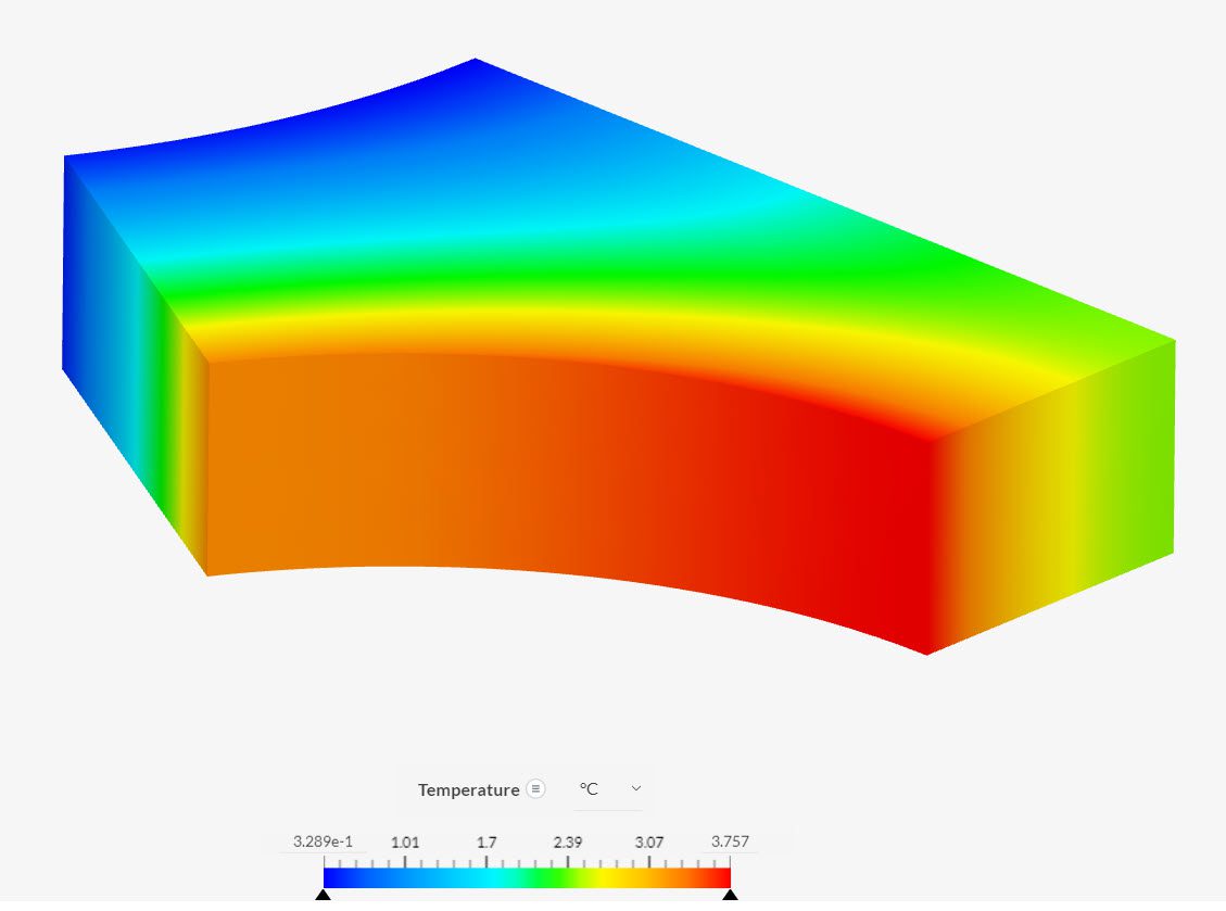
All of the cases are in good agreement with the reference results.
You can see the temperature distribution on the plate for the last time step for Case A below:
Last updated: July 22nd, 2021
Did this article solve your issue?
How can we do better?
We appreciate and value your feedback.


