Validation Case: Heat Transfer in an Electronics Design
This case belongs to solid mechanics. The aim of this test case is to validate the following parameters within the components of an electronics design:
- Transient change in temperature with respect to ambient temperature.
The simulation results of SimScale are compared to the results presented in [Bruce]\(^1\).
Geometry
The geometry used for the case is as follows:
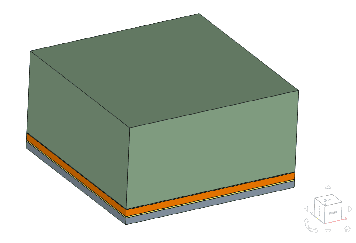
A more descriptive schematic of the components explains the configuration as shown in Figure 2:
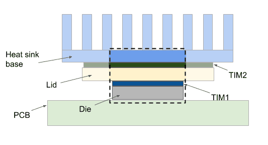
The analysis is carried out on a high-power IC package that is attached between the heatsink base and the PCB substrate. The components explicitly represented in the simulation model are the die, TIM 1, lid, TIM 2, and the heat sink base (where TIM = Thermal Interface Material). These components are shown inside the dashed square box above.
The following table displays the dimensions of each component in the electronics design:
| Component | Length \([mm]\) | Width \([mm]\) | Thickness \([mm]\) |
|---|---|---|---|
| Die | 13 | 13 | 0.50 |
| TIM 1 | 13 | 13 | 0.10 |
| Lid | 13 | 13 | 0.50 |
| TIM 2 | 13 | 13 | 0.05 |
| Heat sink base | 13 | 13 | 6.00 |
Analysis Type and Mesh
Tool type: Code_Aster
Analysis type: Heat transfer, Non-linear
Time dependency: Transient
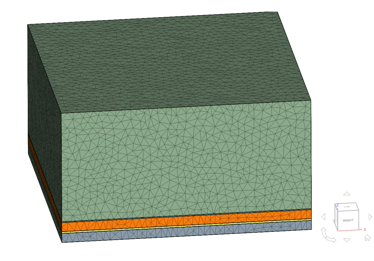
Mesh and element types: SimScale’s Standard algorithm was used to generate the mesh for the electronics design.
| Meshing algorithm | No. of nodes | No. of volumes | Mesh Elements |
|---|---|---|---|
| Standard | 38694 | 184359 | Tetrahedral/Hexahedral |
The final mesh can be seen below:
Simulation Setup
Material:
- Isotropic with the following specifications for each part:
| Component | Material | Thermal conductivity \([ \frac{W}{m\ K}] \) | Density \([\frac{kg}{m^3}]\) | Specific heat \([\frac{J}{kg\ K}] \) |
|---|---|---|---|---|
| Die | Silicon | 111 | 2330 | 668 |
| TIM1 | Ag-Epoxy | 2.0 | 4400 | 400 |
| Lid | Copper | 390 | 8890 | 385 |
| TIM2 | Grease Aluminium filler particle | 1.0 | 2500 | 900 |
| Heat sink base | Copper | 390 | 8890 | 385 |
Initial conditions:
- Temperature \(T\) = 273.15 \(K\)
Boundary conditions:
- Heat flux loads:
- Surface heat flux:
A power of 1 \(W\) is applied to the top surface of the die which is in contact with TIM 1. Therefore, the resulting surface heat flux at this surface is calculated by dividing the power with respect to the die surface area.
Surface heat flux = 1/(169e-6) = 5917.1598 \(W \over \ m^2\) - Convective heat flux:
The cooling effect of the heatsink fins is collectively represented through a heat transfer coefficient that is directly applied to the heatsink base (top surface of the geometry). Therefore, a convective heat flux boundary condition is used to represent the thermal resistance offered by the heatsink to the surrounding air.
Convective heat flux = 20000 \(W \over \ m^2 \ K\)
- Surface heat flux:
Electronics Design Result Comparison
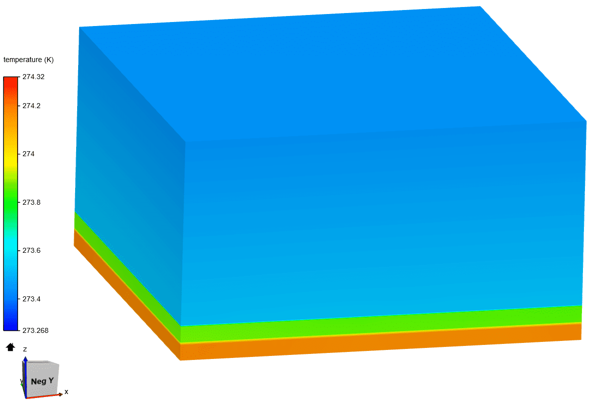
The temperature distribution of the IC package is as shown below:
The comparison of SimScale results with that of [Bruce]\(^1\) for the die, lid, and heat sink is shown below:
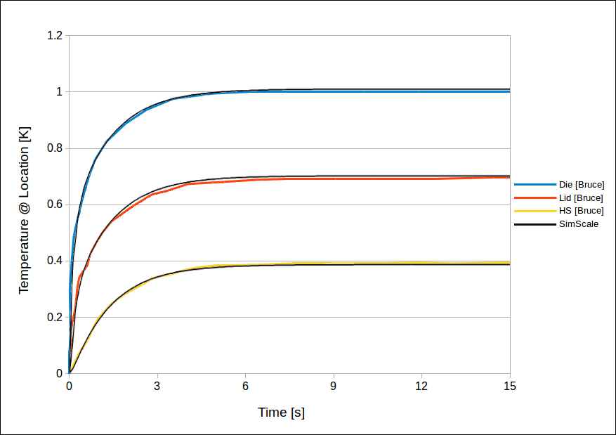
The results are calculated by deducting the initial temperature condition of 273.15 \(K\) from the average temperature value of each area for 150 timesteps.
A slight deviation in the temperature graphs comparison above is due to the approximation error caused during the extraction of temperature values from the digital plots.
Last updated: March 25th, 2026
Did this article solve your issue?
How can we do better?
We appreciate and value your feedback.


