Validation Case: Aerodynamics of the Ahmed Body using LBM Solver

This validation case falls under the domain of fluid mechanics, specifically addressing the aerodynamic characteristics of the Ahmed body. The objective of this study is to assess and validate the following parameters by employing the Incompressible Lattice Boltzmann Method (LBM) by Pacefish®$^2$:

Drag coefficient
Velocity profiles

The simulation results from SimScale were compared to the experimental data presented in the study: S.R. Ahmed, G. Ramm, Some Salient Features of the Time-Averaged Ground Vehicle Wake, SAE-Paper 840300, 1984$^1$

View Project

Geometry

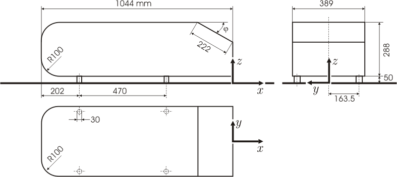
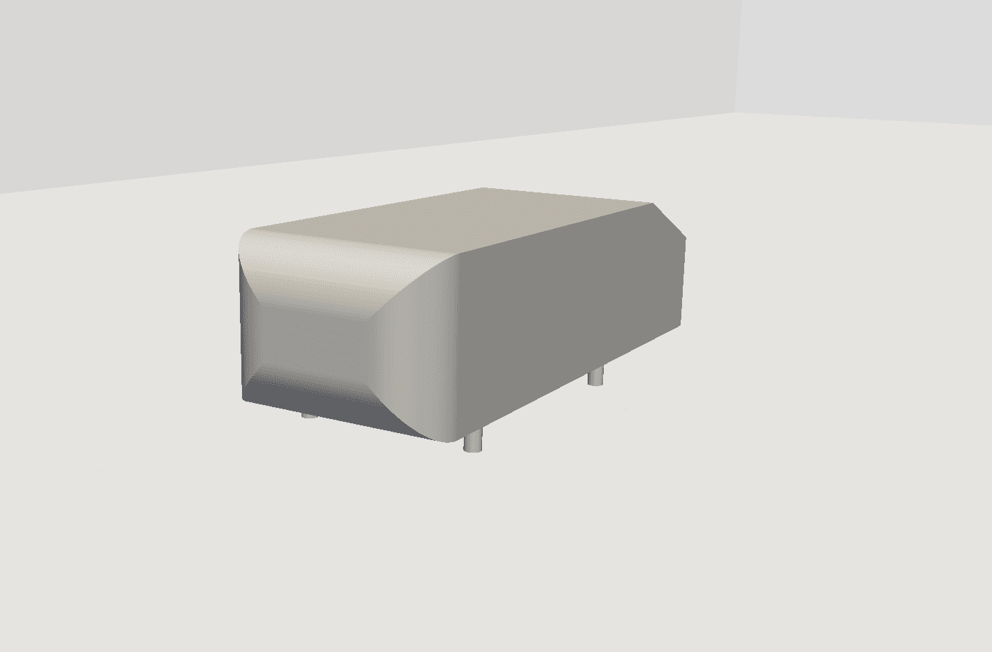
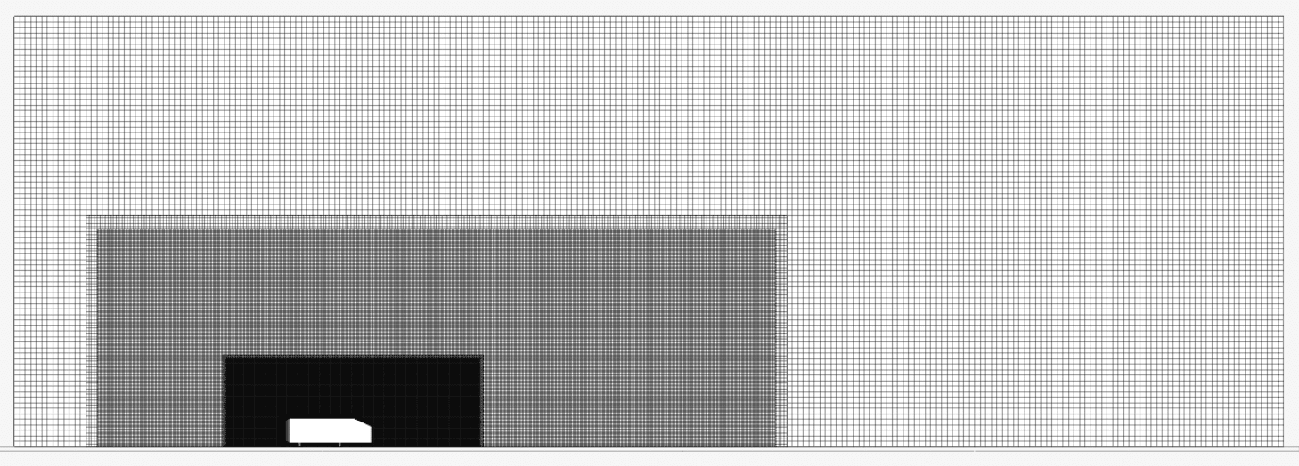
The geometry is created based on the simplified aerodynamic body used by Ahmed et al$^1$. See Figure 1 for dimensions and Figure 2 for the geometry. The slant angle ($\phi$) is set to 25°. The body is placed in a wind tunnel 6 $m$ x 5 $m$ x 13.5 $m$ in order to limit the aerodynamic blockage effect.

ahmed body geometry — Figure 2: Three-dimensional view of the geometry used in the study

Analysis Type and Mesh

Tool Type: Lattice Boltzmann Method (LBM) (Pacefish$^®$ by Numeric Systems GmbH)

Analysis Type: Transient, Incompressible flow with K-Omega SST turbulence model

Mesh and Element Types:

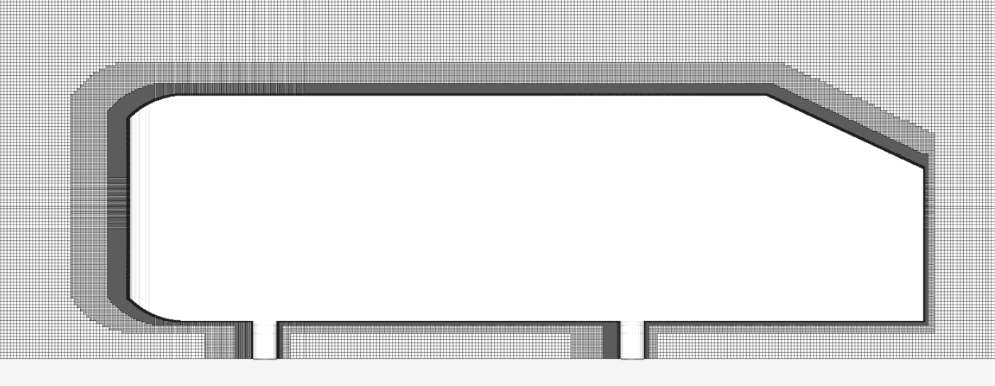
In order to get accurate results, manual mesh settings were applied. The mesh algorithm uses the lattice Boltzmann method, where a Cartesian background mesh is generated, composed only of cube elements that are not necessarily aligned with the geometry of the buildings or the terrain. (see Figures 3 and 4).

ahmed body simulation mesh — Figure 3: Mesh 3 of the three meshes investigated in the Ahmed body validation case

Figure 4: Close-up view of Mesh 3 around the Ahmed body

Three meshes were computed in increasing order of fineness to compute and match the values of drag force with the study$^1$.

The mesh density was consciously increased such that the background mesh remained at the same coarse level, while the surface and region refinements around the car were progressively added. The details are shown in Table 1.:

Mesh	Background mesh (Manual)	Car surface Refinement $[m]$	Region Refinement 1 $[m]$	Region Refinement 2 $[m]$	Number of Cells
Mesh 1	Very Coarse	0.005	0.015	0.02	21 282 816
Mesh 2	Very Coarse	0.002	0.01	0.02	50 016 640
Mesh 3	Very Coarse	0.0008	0.006	0.02	182 706 176

Table 1: Mesh details for three different meshes. The value for refinements represent the target resolution in meters.

Note

Further mesh refinements were discarded due to extremely high mesh cell count and no improvement in the drag force value observed.

Simulation Setup

Material

Fluid

Air
- Kinematic viscosity $(\nu)$: 1.5 x 10^-5 $kg/ms$
- Density $(\rho)$: 1.196 $kg/m^3$

Boundary Conditions

When using the LBM solver, the boundary conditions are assigned on the faces of the flow domain.

The boundary conditions for the simulation are shown in Figure 5 below:

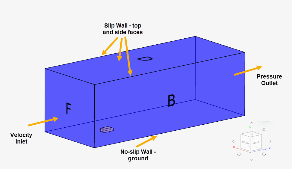
ahmed body boundary conditions — Figure 5: Boundary conditions applied to the faces of the Ahmed body fluid domain. Not all associated face names are visible.

Details of the applied boundary conditions are further discussed below:

Face	Boundary Condition	Value
F	Velocity inlet – Fixed Magnitude Turb. kinetic energy Specific dissipation rate	60 $[m/s]$ 0.135 $[m^2/s^2]$ 180.1 $[1/s]$
E	Pressure Outlet	–
A, B, D	Slip Wall	–
C	No-slip Wall

Table 2: Boundary conditions for each face of the external flow domain

The free stream velocity of the simulation is 60 $m/s$, so that the Reynolds number based on the length of the body $L$ is 4.29e6. Those are the same values presented in the original experiment of Ahmed and Ramm$^1$.

Simulation Control

The simulation is transient in nature and was run to simulate a real time of 0.4 seconds. This ensures that the air flow passes a ~2 times over the Ahmed body, given the flow domain size, and the inlet velocity. Due to the stable nature of the solution, longer times were discarded to save computational expenses.

Reference Solution

The experimental solution is presented in Figure 4 in the reference paper$^1$, giving the value for the drag force coefficient for the slant angle $\phi$ = 25°:

$$ C_{d} = 0.2875 $$

Result Comparison

Drag Coefficient

The drag force is defined as

$$ F_{d}={\frac {1}{2}}\rho \,U^{2}\,C_{d}\,A_x $$

where $A_x$ (0.115 $m^2$) is the projected area of the Ahmed body in the streamwise direction and $F_{d}$ the drag force. The drag force and drag coefficient were determined by the integration of surface pressure and shear stress over the entire Ahmed body (except for the 4 stilts acting as support).

The resulting drag coefficient of the Ahmed body, closest to the reference solution as yielded by Mesh 3, was computed to be 0.2997, which is within a 4.71 % error margin of the experimental value.

Table 2 shows the result of the mesh independence study:

Mesh	DRAG FORCE $[N]$	DRAG COEFFICIENT	REFERENCE	ERROR [%]
Mesh #1	94.31	0.3879	0.2875	32.5
Mesh #2	76.66	0.3096	0.2875	7.7
Mesh #3	74.53	0.2997	0.2875	4.71

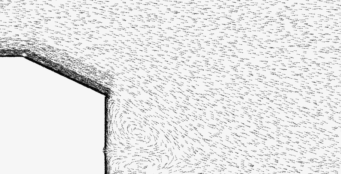
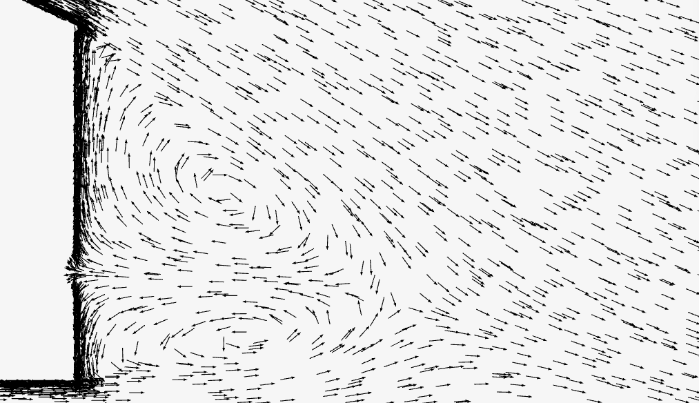
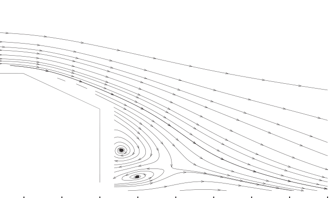
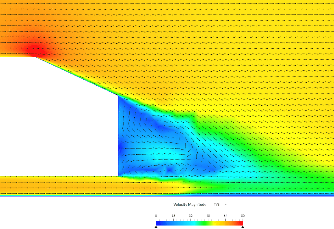
Table 2: Results comparison and computed errors between 3 different meshes

Wake Flow Patterns

The velocity streamline contour of the mean flow obtained with the simulation is reported in Figures 6 and 7, together with experimental results for reference in Figure 8.

recirculation pattern at the back of the ahmed body — Figure 6: Velocity vectors in the suction region behind the car plotted within SimScale’s online post-processor

close up of the recirculation pattern at the back of the ahmed body — Figure 7: A close-up view of the flow as described in Figure 6, emphasizing flow detachment and creating a “rear vacuum” along with two primary vortices.

ahmed body wake experimental results — Figure 8: Experimental results for comparison showing a schematic of the streamlines over the Ahmed body

References