Tutorial: Fluid Flow Through a Pipe Junction

This article provides a step-by-step tutorial for a fluid dynamic simulation of a pipe junction.

pipe junction tutorial incompressible flow — Figure 1: Particle traces through a pipe junction

Overview

Simulating pipe junctions can be useful to understand delta pressures through the system, check whether recirculation regions arise, and observe how the flow mixes. This tutorial contains a simple workflow with the Incompressible solver to simulate pipe junction cases.

We are following the typical SimScale workflow:

Preparing the CAD model for the simulation.
Setting up the simulation.
Creating the mesh.
Run the simulation and analyze the results.

1. Prepare the CAD Model and Select the Analysis Type

First of all, click the button below. It will copy the tutorial project containing the geometry into your Workbench.

Import tutorial into Workbench

The following picture demonstrates what should be visible after importing the tutorial project.

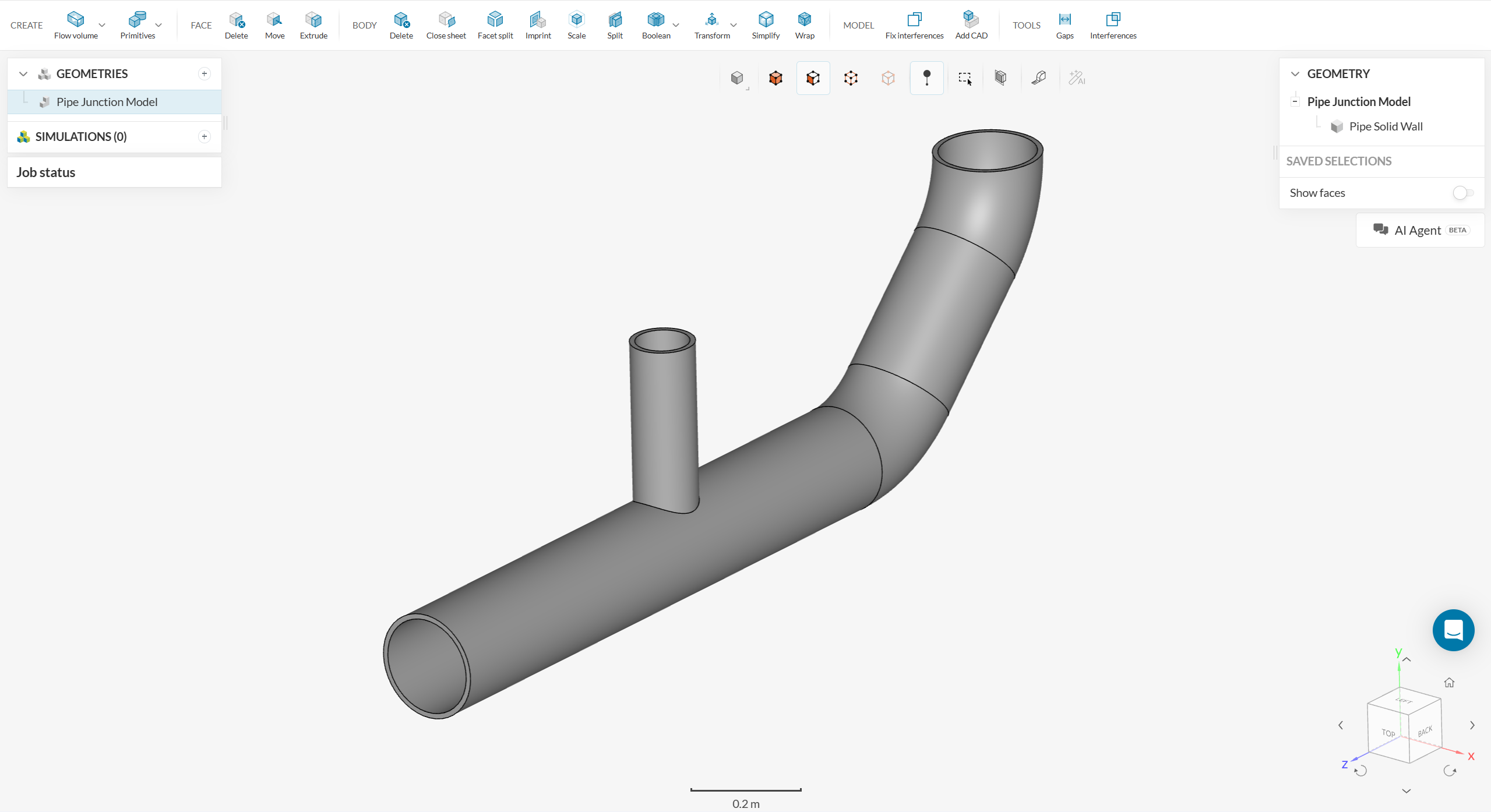
import view pipe junction tutorial — Figure 2: Initial CAD model, containing the solid walls of the pipe

1.1 Editing the CAD Model

The initial CAD model contains the solid walls of the pipe but not the volume occupied by water. As such, before setting up the simulation, a Flow region, representing the fluid domain, needs to be created.

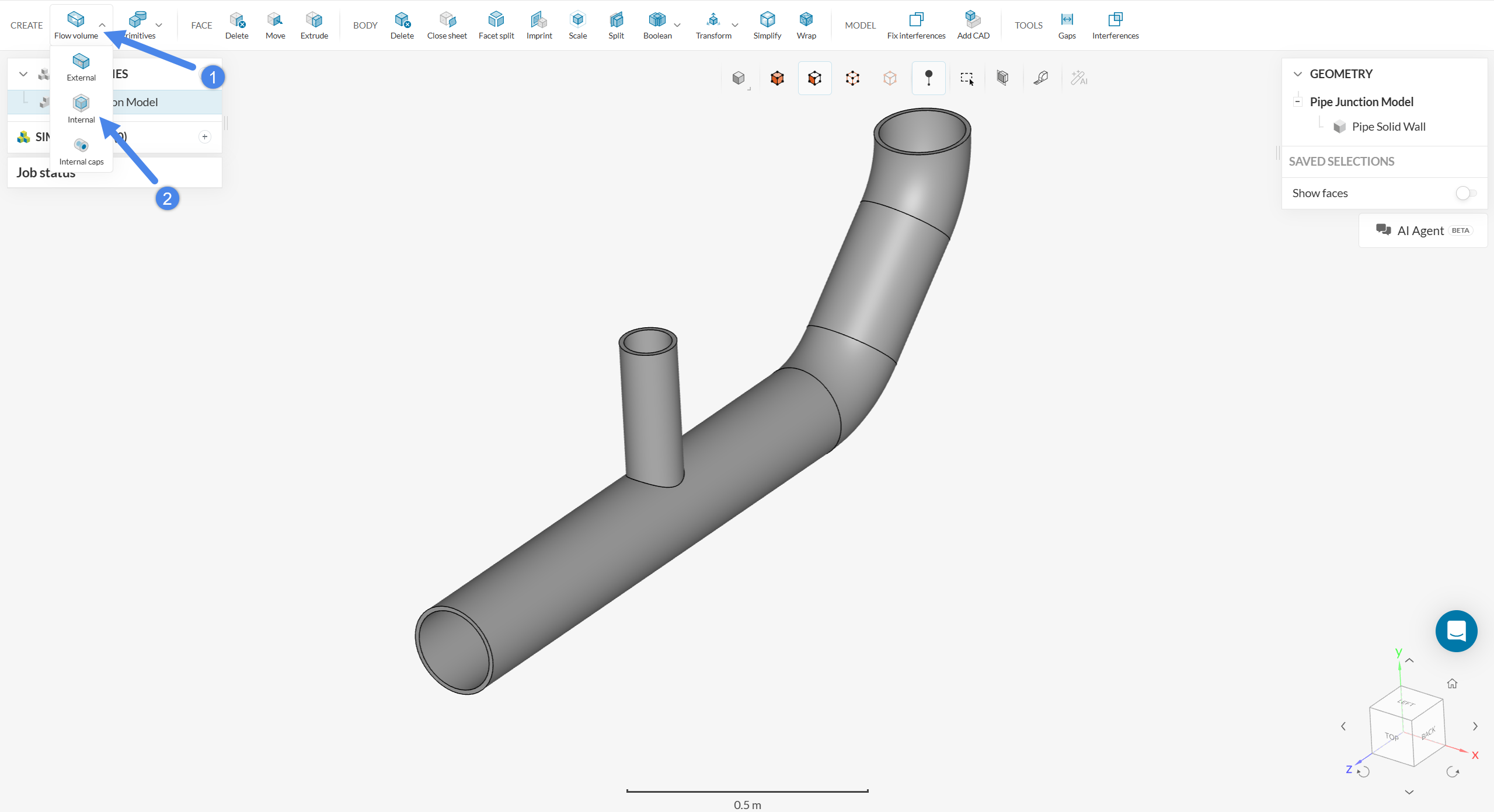
Since the flow region is internal to the pipe, select an ‘Internal’ flow volume operation:

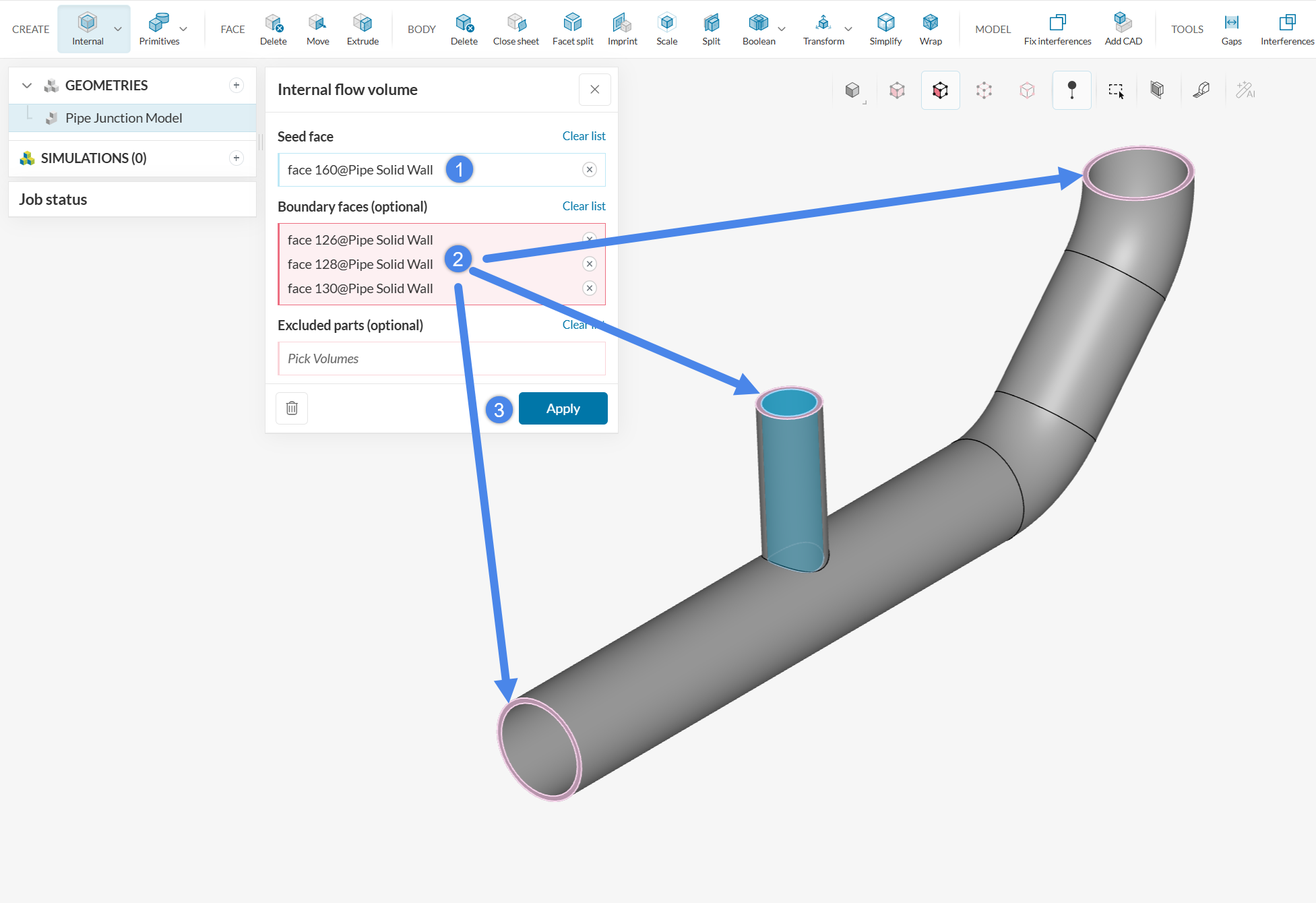
tutorial 2 creating flow region — Figure 3: Creating an internal flow region to represent the water domain inside of the pipe

In the internal flow region setup window, seed and boundary faces have to be assigned for this model. Since the tube has 3 openings, there will be 3 boundary faces in pink, below. The boundary faces cover the openings of the tube.

For seed face, only one assignment is needed. It can be any wetted face, so any face in contact with the flow region that we are looking to create works (i.e. a face on the inside of the pipe). Press ‘Apply’ once you assign the faces.

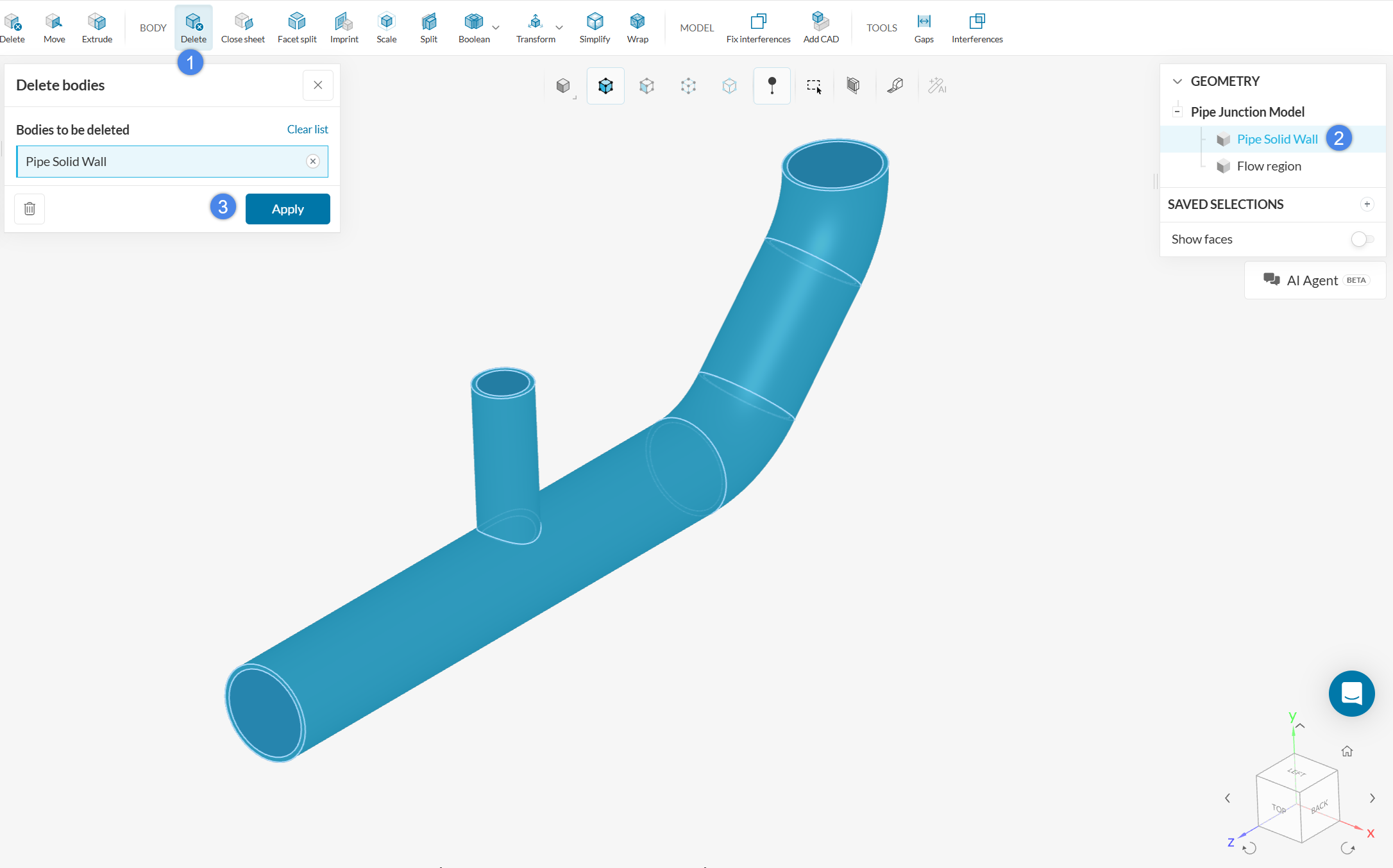
flow volume creation for a pipe — Figure 4: Creating a flow region for a pipe geometry. Note that the seed face needs to be one of the internal pipe faces.

As discussed, this tutorial will use the Incompressible solver. With this solver, the geometry must contain a single flow region volume, and no solid materials are allowed. As such, we will delete the solid walls of the pipe with a ‘Delete’ body operation:

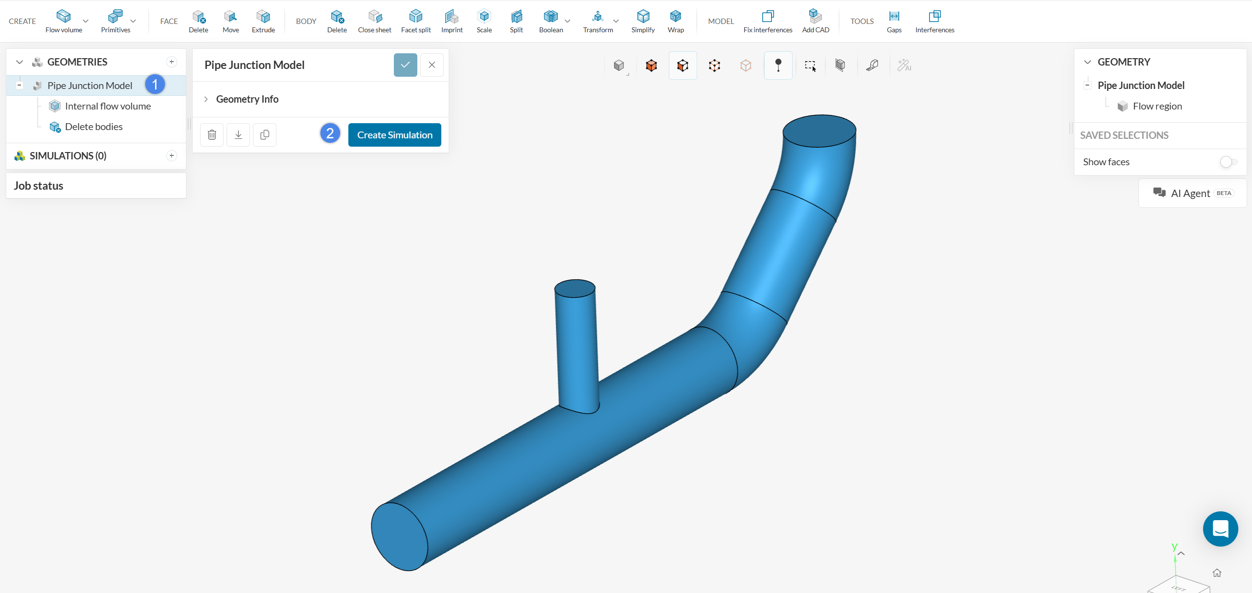
deleting solid parts in an incompressible study — Figure 5: Incompressible analyses, such as the one from this tutorial, require a CAD model with a single flow region.

1.2 Create a Simulation

By the end of the CAD operations, the CAD model should contain a single volume, representing the flow region. At this point, to create a new simulation, select the geometry and click the ‘Create Simulation’ button.

creating a new incompressible analysis of a pipe — Figure 6: Creating a new simulation in SimScale

In doing so, the analysis type selection widget opens up. Choose ‘Incompressible’ from the list and click on ‘Create Simulation’.

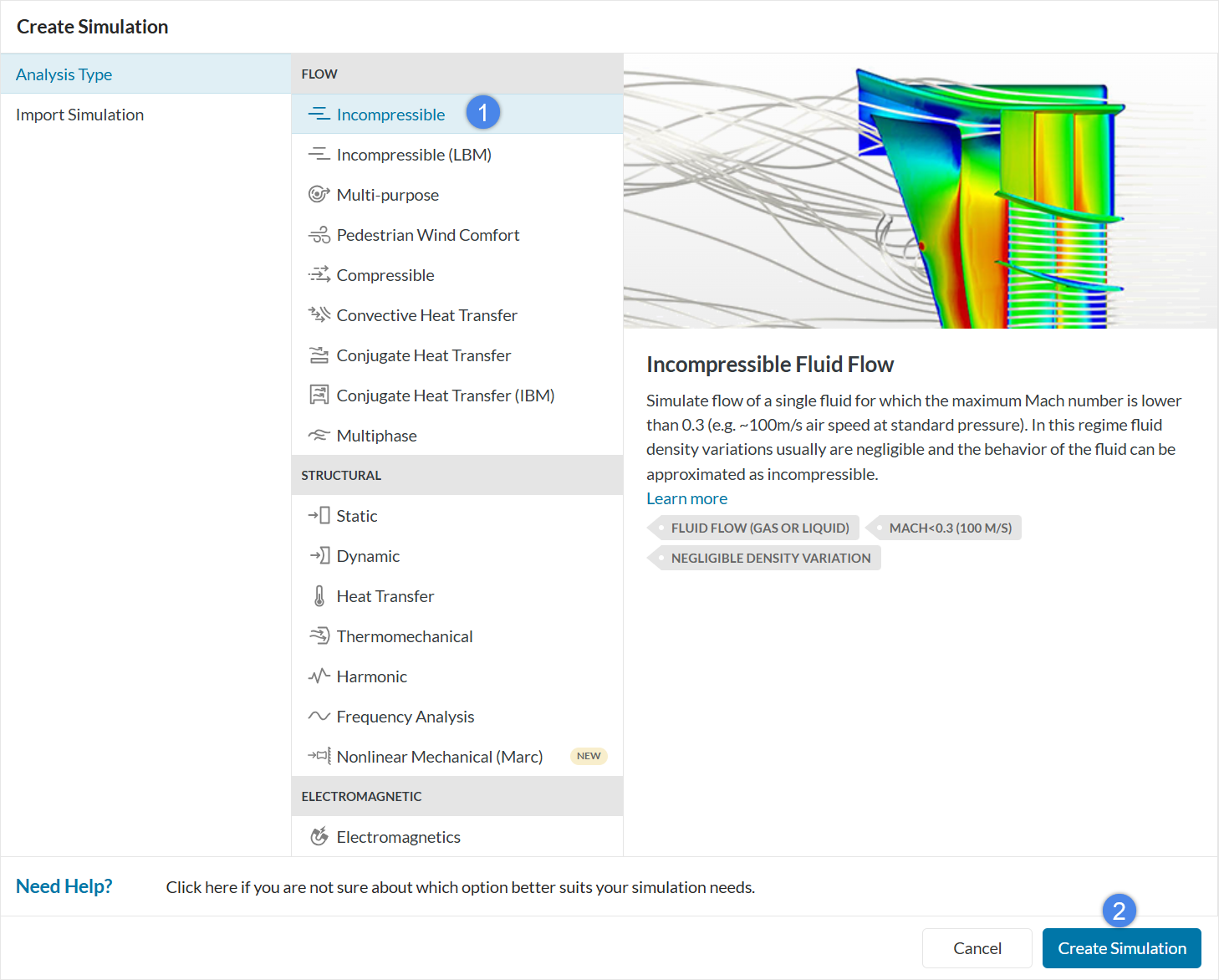
creating an incompressible simulation in simscale — Figure 7: From the analysis selection widget, choose ‘Incompressible’.

Incompressible analyses are isothermal and better suited for low speed flow (Mach Number below 0.3), which is the case for this tutorial.

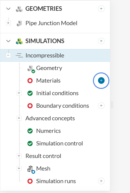
2. Assign Materials and Boundary Conditions

2.1 Define a Material

To assign a new material, click on the ‘+’ button next to Materials in the simulation tree.

creating a new simulation in simscale — Figure 8: Creating a new material in the simulation tree

This will open the Material library which contains all the available materials for a simulation. Scroll down to select ‘Water’ and click ‘Apply’.

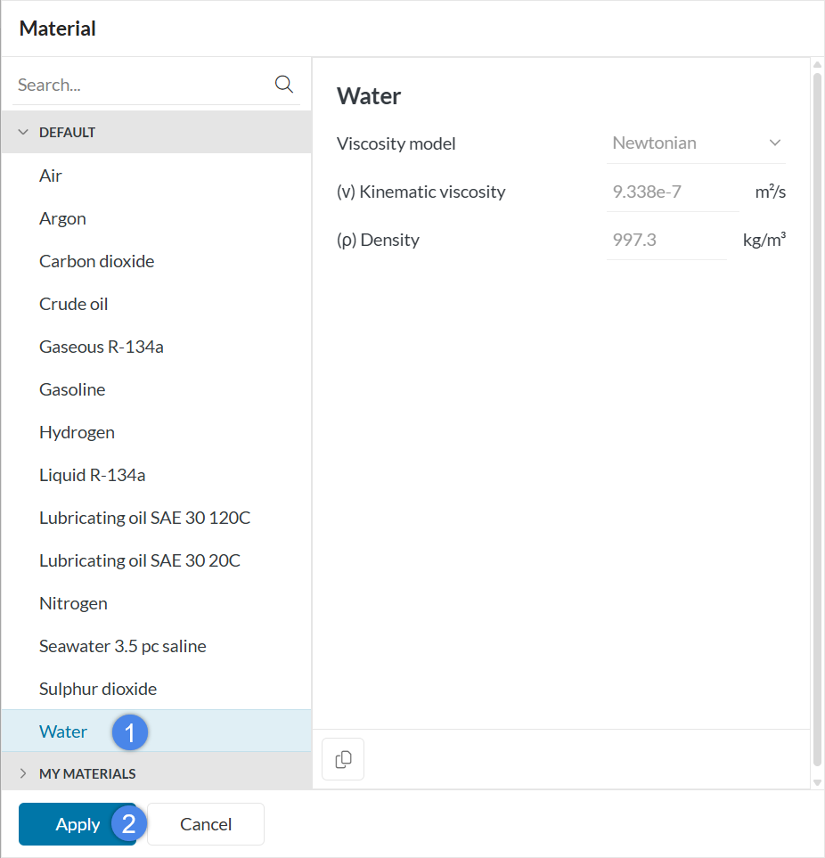
default list of materials simscale — Figure 9: Choose ‘Water’ from the list of materials

Water will be automatically assigned to the flow region.

2.2 Assign Boundary Conditions

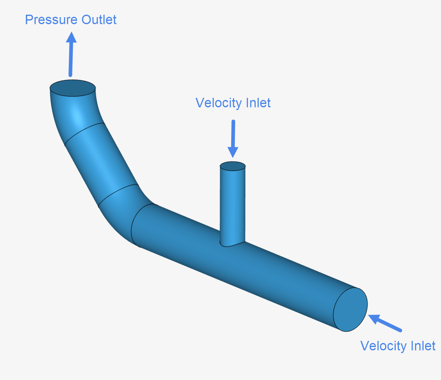
Boundary conditions are constraints that define the physical boundaries of the simulation, such as the input and output of a pipe. For this simulation, three boundary conditions will be necessary so that we can model water meeting at the junction of the pipe coming from the horizontal and vertical inlets.

boundary condition overview in the setup — Figure 10: Boundary condition overview for the pipe flow tutorial

a. Velocity Inlets

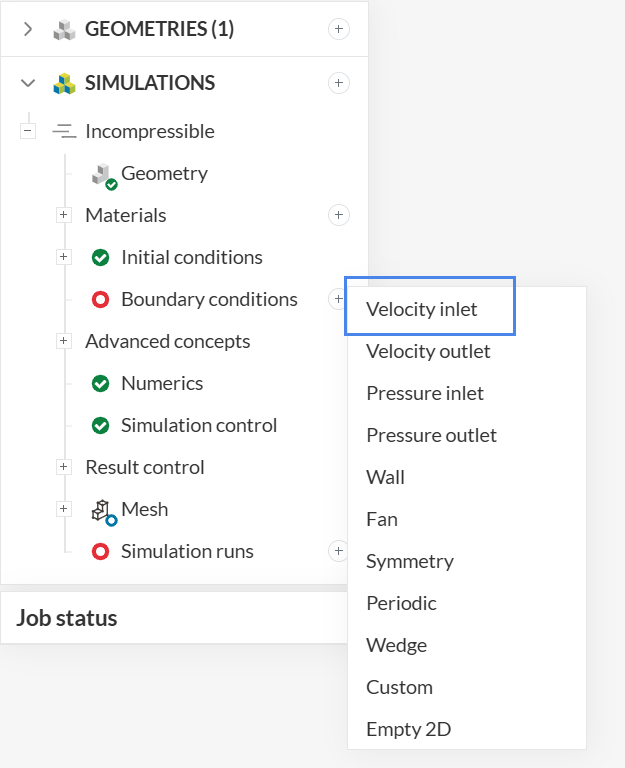
To create a new boundary condition, click on the ‘+’ button next to Boundary conditions in the simulation tree. Select ‘Velocity inlet’ from the list.

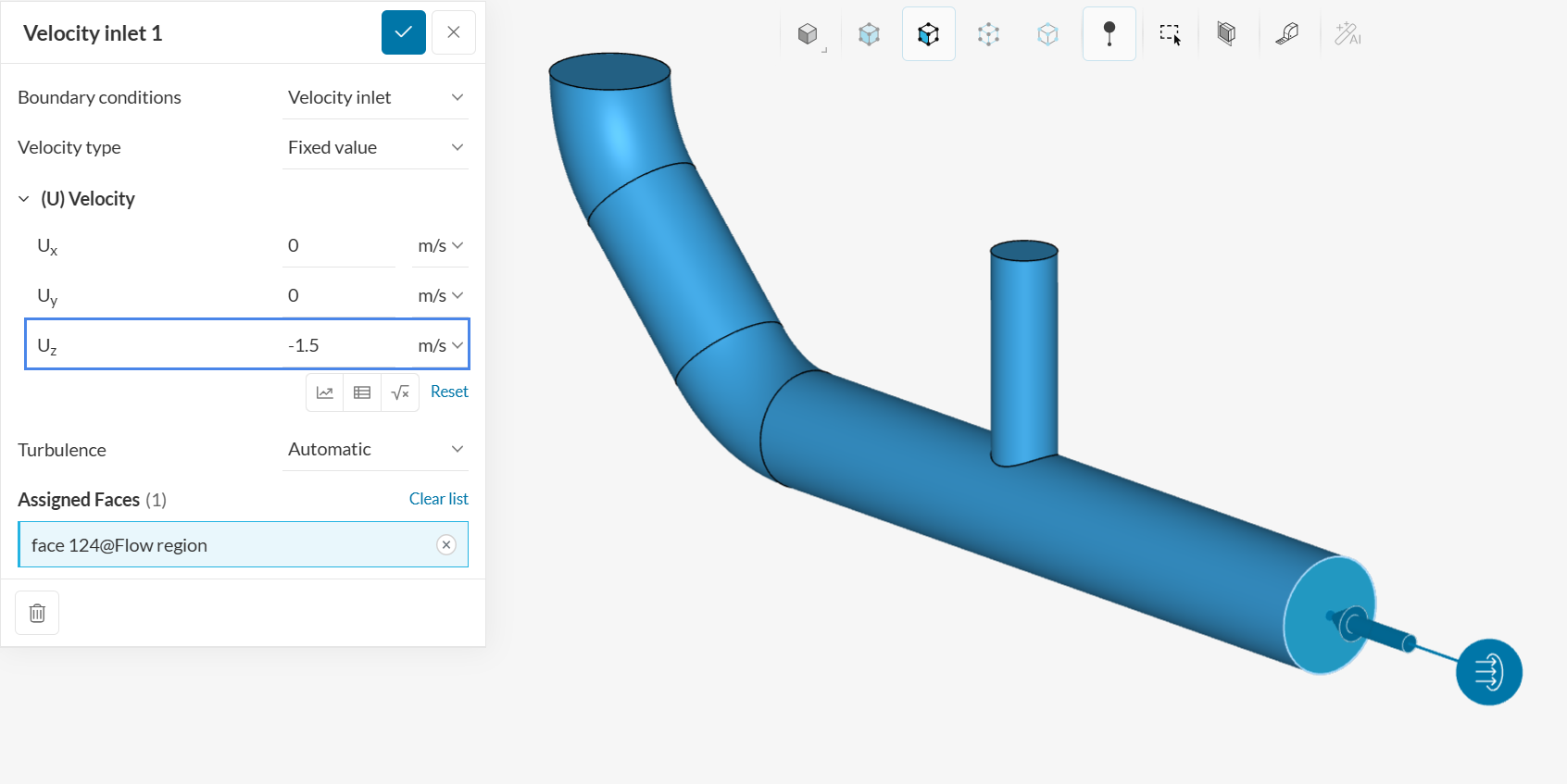
boundary condition creation — Figure 11: Creating boundary conditions in the simulation tree

In the velocity inlet setup window, set the velocity in z-direction to ‘-1.5’ \(m/s\). This will assign a flow with the specified velocity to the assigned face. In this case, flow from the negative z-direction is needed to model the horizontal flow. The global coordinates can be found in the viewing cube at the bottom right of your screen.

Select the horizontal face in the viewer. This will assign the face as a velocity inlet.

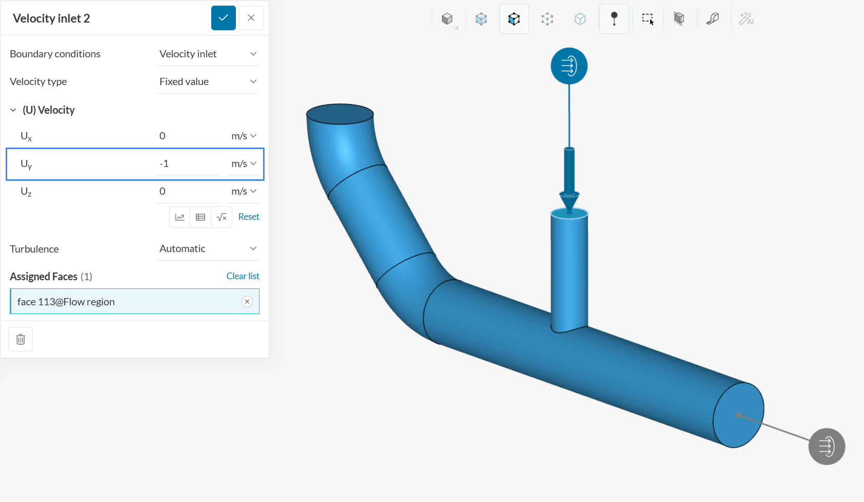
boundary condition for inlets — Figure 12: Setting up a velocity inlet boundary condition to the main inlet face.

We will set up another velocity inlet to simulate a vertical flow by following the same steps as before. Set the velocity in y-direction to ‘-1’ m/s. Select the face to assign the new velocity inlet.

multiple velocity conditions — Figure 13: Secondary velocity inlet boundary condition.

b. Pressure Outlet

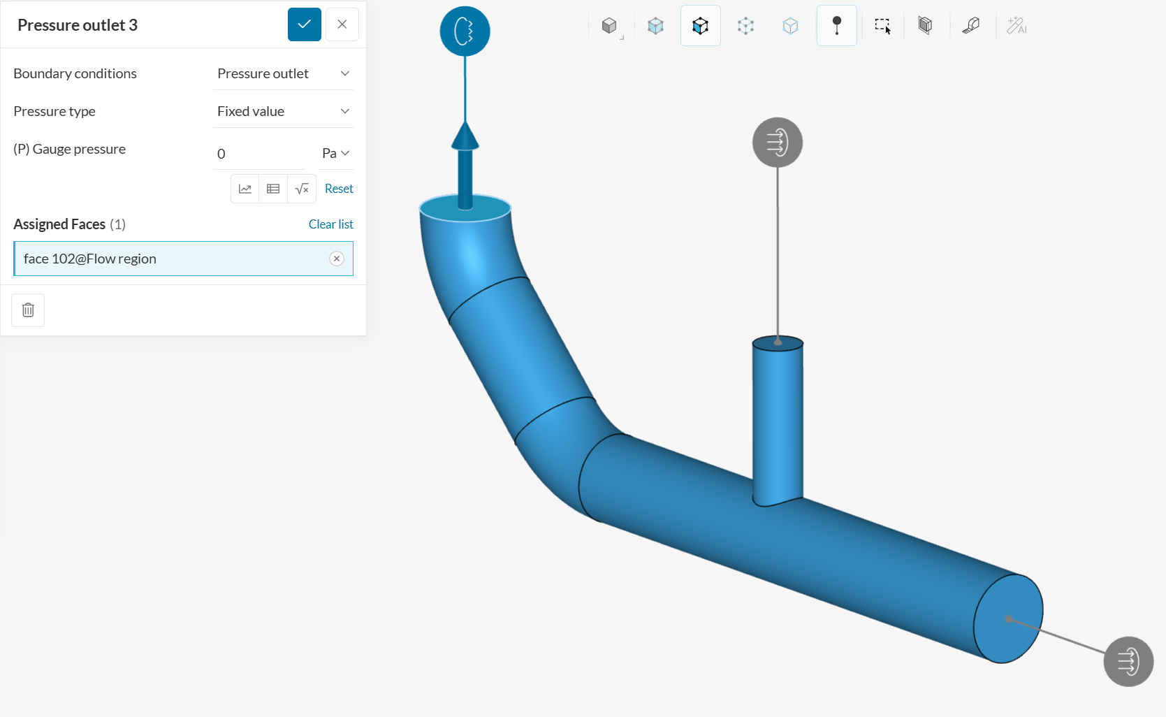
Last but not least, we will add a third boundary condition which is the ‘Pressure outlet’, indicating the face where the fluid will leave the domain. Select the face below to assign it as a pressure outlet boundary condition.

pressure outlet boundary condition pipe flow — Figure 14: Setting up a pressure outlet boundary condition for pipe flow

2.3 Result Control

Please navigate to Result control in the simulation tree to set up an ‘Area average’ monitor within Surface data:

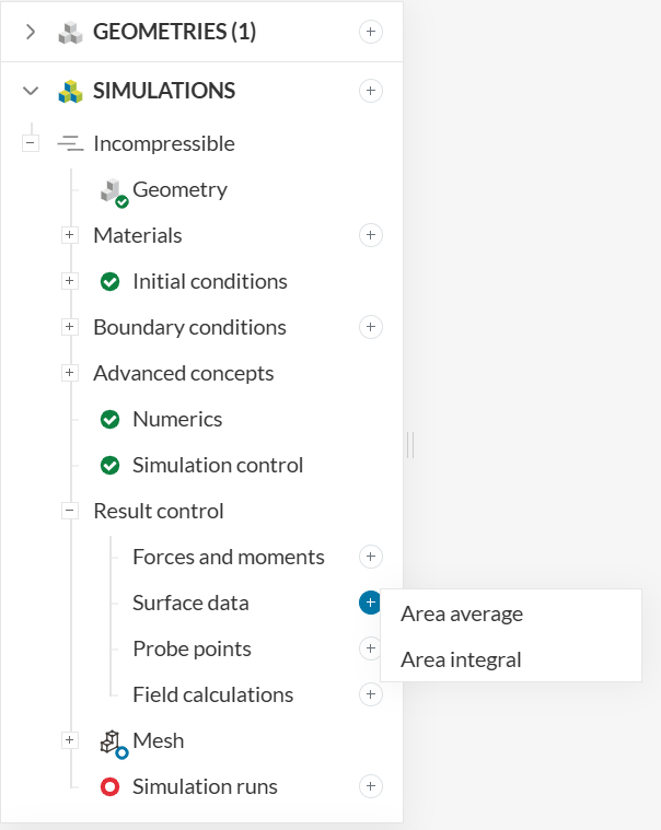
creating result controls in simscale — Figure 15: Result controls are useful to evaluate the convergence of a simulation

In this simulation, let’s keep track of the inlet values with an area average:

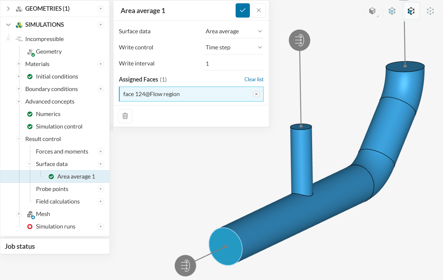
result control monitoring inlet average values — Figure 16: Assign the area average result control to the horizontal inlet.

For pipe flow, monitoring the inlet faces also helps to evaluate pressure losses through the system.

3. Mesh and Simulation

This tutorial will use a single-click simulation workflow. Instead of generating a mesh and then running the simulation, we will proceed to running the simulation directly.

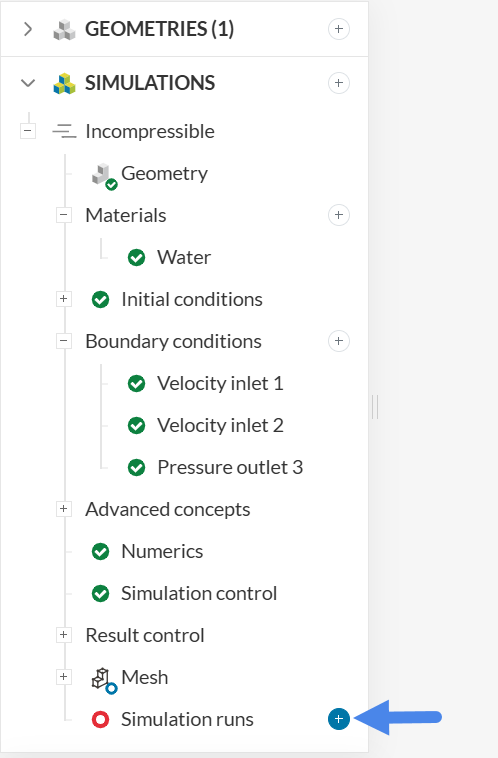
In the background, SimScale will generate the mesh and, as soon as it is finished, the simulation will start automatically. As such, create a simulation run by clicking on the ‘+’ button next to Simulation runs in the simulation tree.

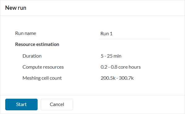
starting a simulation run in simscale — Figure 17: You can start a simulation by clicking on the ‘+’ button.

A dialog box will appear stating the estimated amount of resource consumption. Click ‘Start’ in the New run dialog box to start the simulation run.

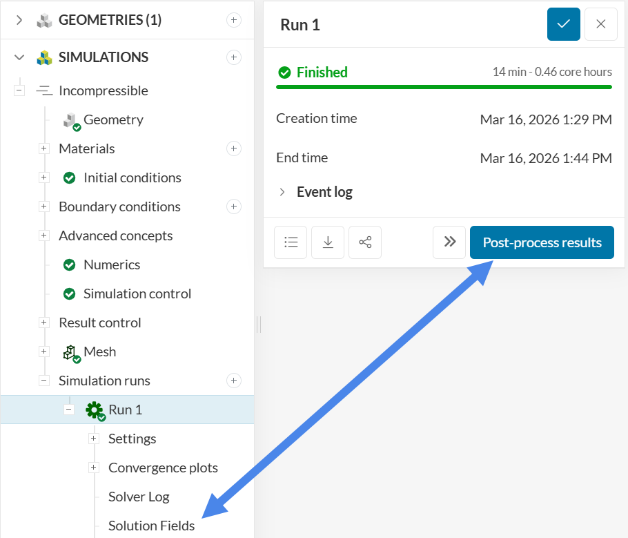
new simulation window — Figure 18: New run dialog with resource estimate for pipe junction flow simulation

Once the simulation run is finished, the status will be changed to Finished in the run settings panel.

Did you know?

In SimScale you may also generate and inspect the mesh before running the simulation. To do that, go to Mesh and click on ‘Generate’. Once the mesh is finished, you can create a simulation run using it.

4. Post-Processing

While the simulation is running, you can inspect the result control values live. From a convergence perspective, it is important that physical quantities of interest stabilize as the simulation progresses. For example, monitoring pressure at the inlet is important for studies involving pressure loss evaluations:

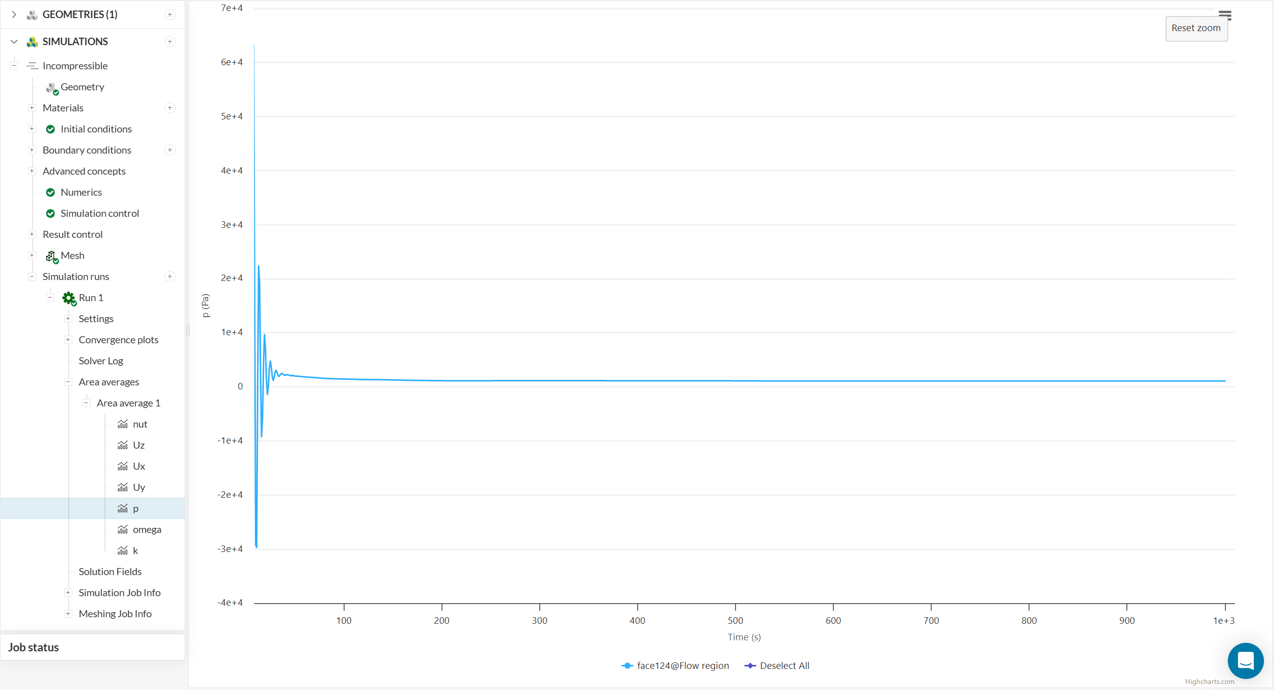
pressure inlet values — Figure 19: Analyzing pressure values at the inlet via result controls.

From the image above, we can see that the pressure at the inlet is very stable after 600 iterations, indicating a good convergence pattern.

Click ‘Post-process results’ or ‘Solution Fields’ under the run to open the post-processor. SimScale’s integrated post-processor consists of filters and different viewing tools to better visualize and download the simulation results.

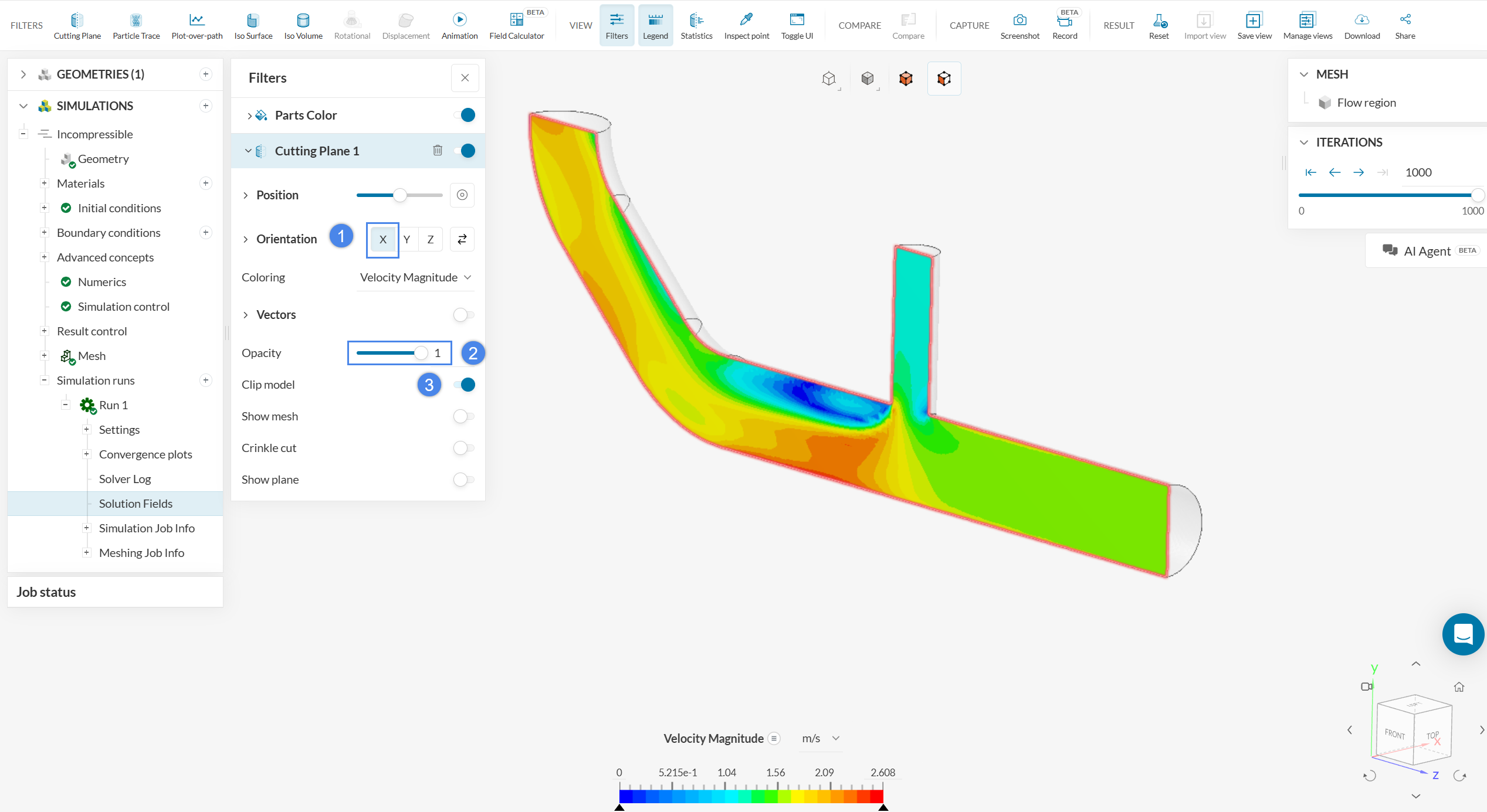
opening simulation results in simscale — Figure 20: How to get to SimScale’s post-processing environment

After opening the post-processor, a cutting plane will be automatically applied. Now, we want to show the flow inside the pipe. Therefore, we will change the orientation of the plane to the x-axis by clicking on ‘X’ besides Orientation. Also, make the cutting plane fully opaque by setting the Opacity to ‘1’, and enable Clip model.

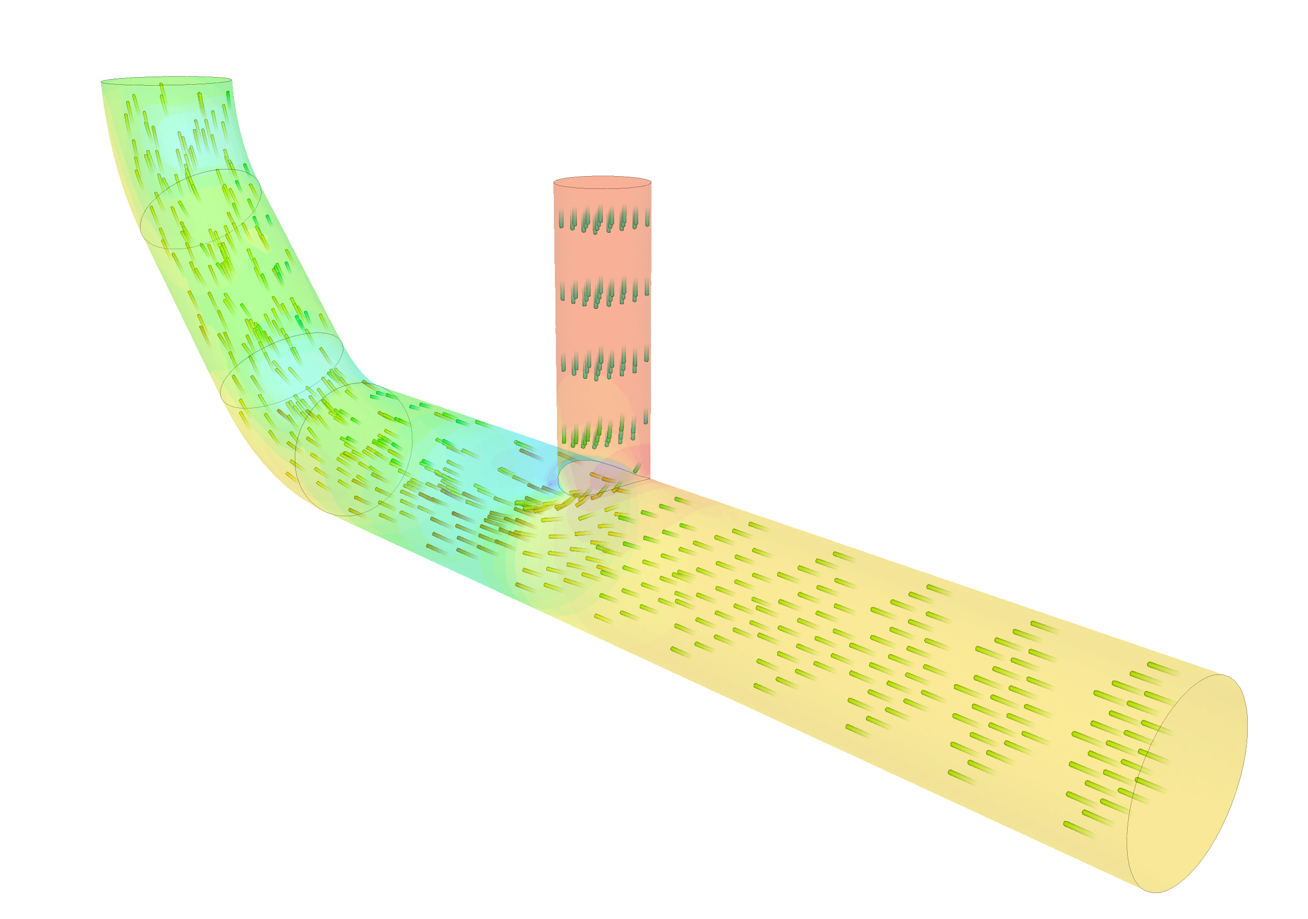
cutting plane creation in the post-processor — Figure 21: Pipe flow junction cut in half with cutting plane in the x-plane to show the velocity magnitude contours inside the pipe junction

You can also find areas where re-circulation occurs by visualizing the velocity vectors as shown below. Turn on the toggle beside Vectors to show the velocity vectors. Next, to make the vectors more clear, you can set the color of the vectors to black beside Coloring.

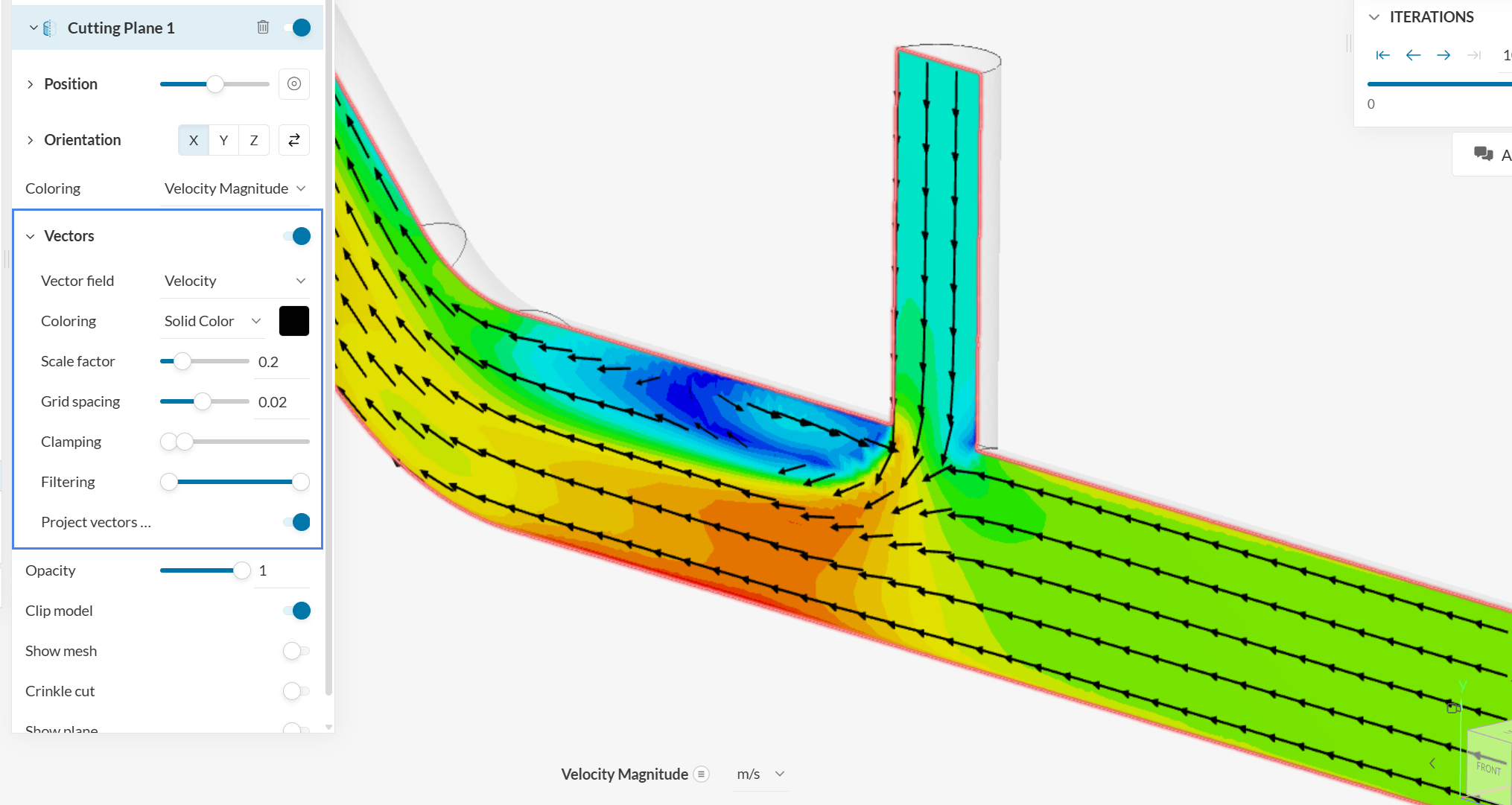
plotting vectors on a cutting plane — Figure 22: Velocity vector settings to help show re-circulation areas

Based on the velocity vectors, we can see a large re-circulation region in the areas near the junction, so this is a region that may require some improvements.

For additional post-processing workflows involving this pipe junction model, make sure to visit this page, which shows examples of all filters and additional post-processing tools.

Congratulations! You finished the tutorial!

Have a look at the finished project

Last updated: March 16th, 2026

Did this article solve your issue?

How can we do better?

We appreciate and value your feedback.