Advanced Tutorial: Internal Thermal Comfort of a Car

This article provides a step-by-step tutorial for the full thermal comfort assessment inside a car using CFD simulation, including models for convective heat transfer and radiation heat transfer.

Overview

This tutorial teaches you how to:

• Set up and run a convective heat transfer flow simulation.
• Assign boundary conditions, material, and other models to the simulation.
• Mesh the geometry with the SimScale standard meshing algorithm.
• Set up radiation heat transfer.
• Define thermal comfort parameters computation.

The typical SimScale workflow will be followed:

1. Prepare the CAD model for the simulation.
2. Set up the simulation.
3. Set up the mesh.
4. Run the simulation and analyze the results.

1. Prepare the CAD Model and Select the Analysis Type

First of all, click the button below. It will copy the tutorial project containing the geometry into your own Workbench.

Figure 1 demonstrates what should be visible after importing the tutorial project.

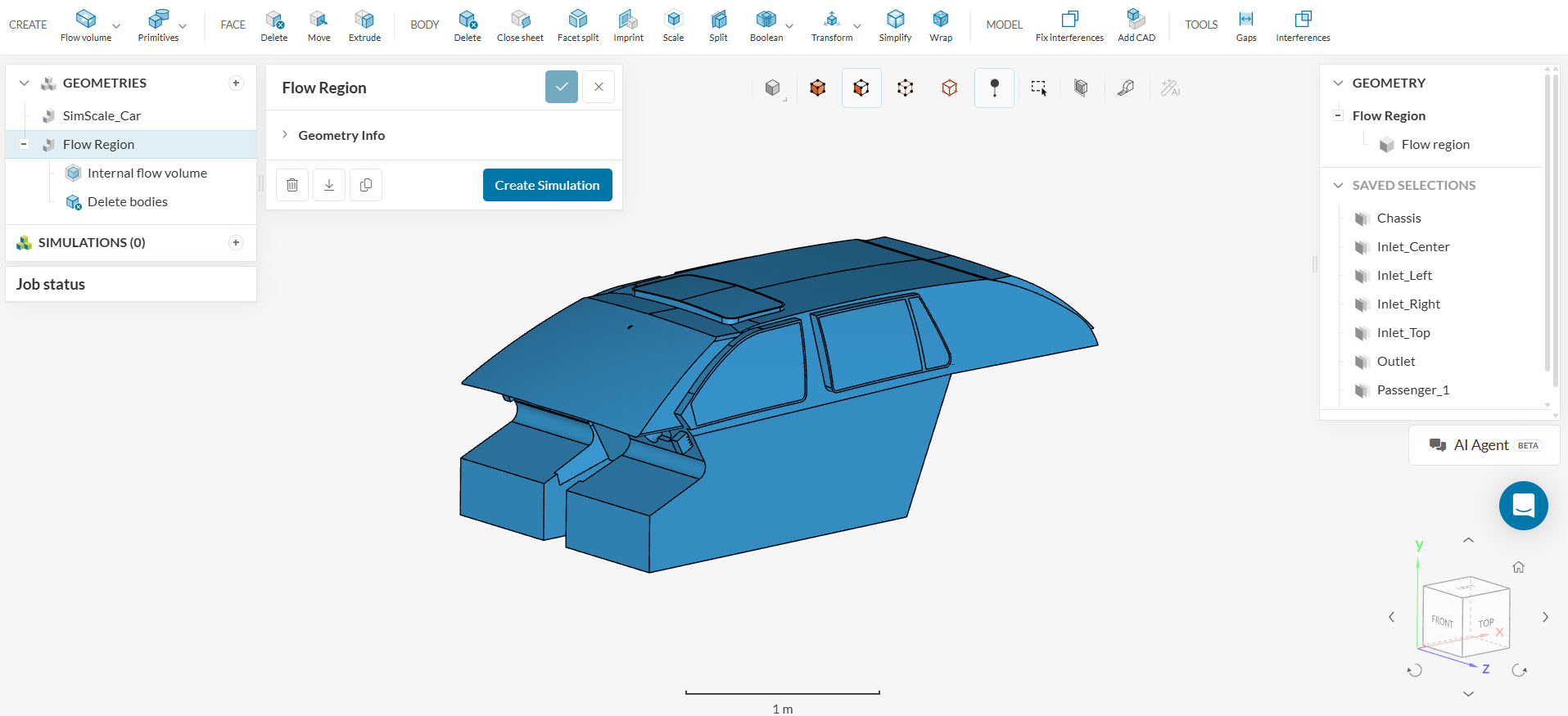
Please notice how the Car_Internal_Volume geometry consists only of one flow region.

The original CAD model, SimScale_Car, included the car, passengers, and a rear mirror. Therefore an Internal flow volume operation was performed in CAD mode. This created the geometry for the volume of air. The volume of air represents the negative of the car cabin and everything inside. Also, note that SimScale_Car was highly defeatured before the import. As an example, all the buttons of the center console have been removed.

1.1 Create the Saved Selections

In the beginning, we want to finish the geometry preparation by setting up the last missing saved selection. Saved Selections are groups of faces, created after the geometry import by the user, to be used in assignments for boundary conditions and other concepts, during the simulation setup. They can be found at the right-hand side panel:

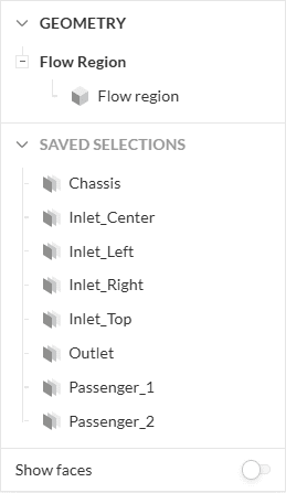
A number of saved selections are already provided in the project, but the saved selection for the windows is still missing. Figure 3 below shows how to add one:

1. Create the entity set by first selecting the faces representing the windows of the car (highlighted in red),
2. then the ‘+’ icon at the left of Saved Selections in the right panel.

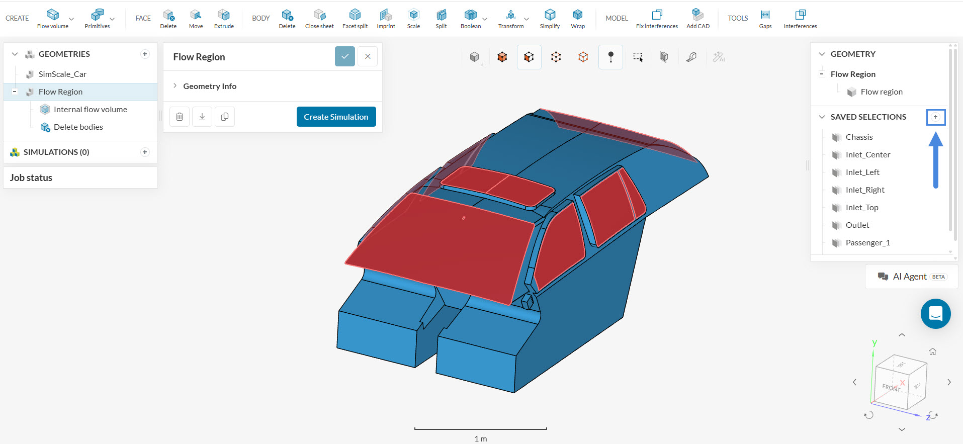
In the pop-up dialog that appears, name the set ‘windows’ and click ‘Create new set‘.

1.2 Create the Simulation

Now we can start with the simulation setup. We will create a new simulation with the ’Conjugate Heat Transfer v.2’ analysis type. This analysis type supports convective and radiational heat transfer and gives us faster solver time compared to the Convective Heat Transfer.

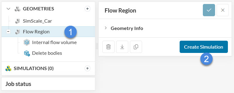
Follow the steps presented in Figure 4 to create a new simulation:

1. Select the ‘Car_Internal_Volume’ geometry under the Geometries panel,
2. Then click the ‘Create Simulation’ button of the dialog:

The simulation library window appears:

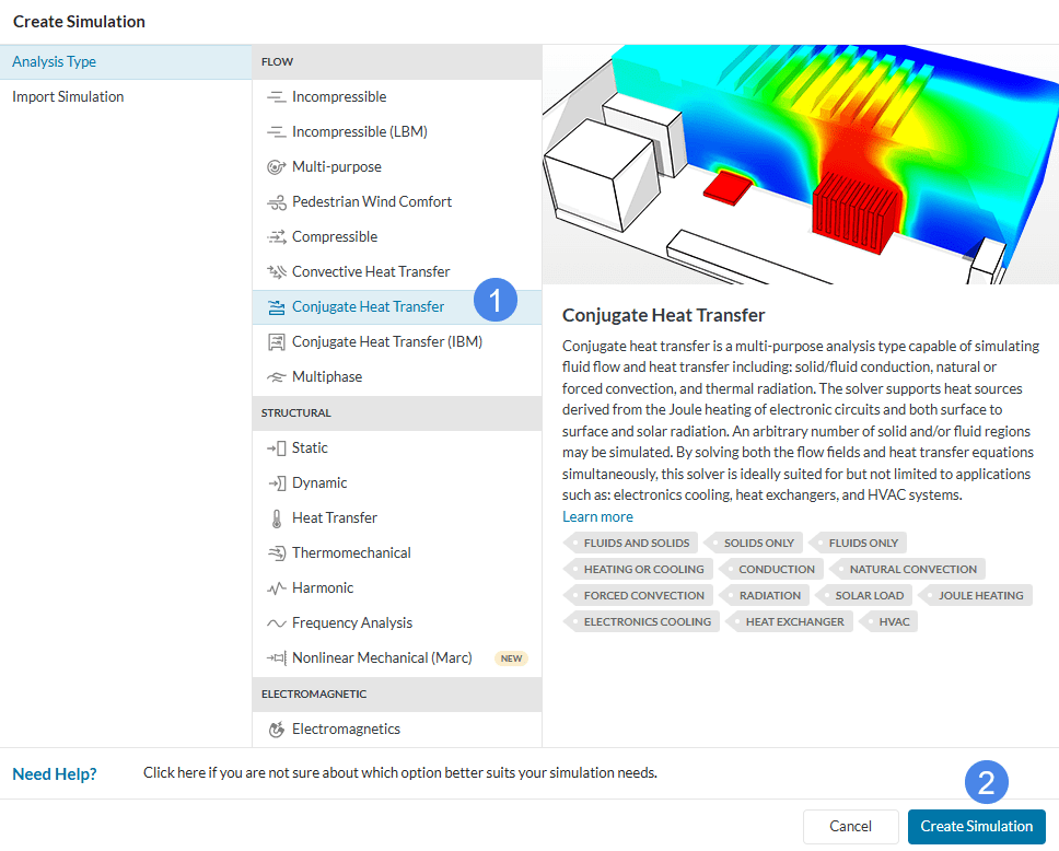
Here you can select the analysis type you need.

3. Choose ‘Conjugate Heat Transfer V2’ and click ‘Create Simulation‘.

Now, you will see the default global settings dialog box opens. Here we can select general settings for the simulation such as the turbulence model or activate certain behaviors of the simulation.

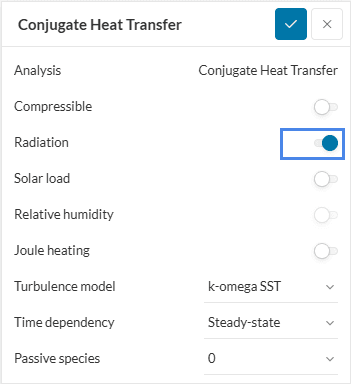
Perform the following changes:

1. Activate Radiation for the simulation.
2. Change the turbulence model to ‘k-omega SST’.

Do not forget to click the checkmark at the top to save the changes

2. Set Up the Simulation

In order to have an overview, the following is a description of the simulation model and conditions. These will later be used to define the boundary conditions of the simulation:

1. Heat transfer is performed through forced convection, natural convection, and radiation, within the fluid domain.
2. Ambient conditions for summer with an ambient temperature of 35 \(°C\) and relative humidity of 65 %.
3. Inlet flow of 27 \(L/s\) through all inlets combined at 19 \(°C\).
4. Outlet flow through the rear opening. 
5. Radiation through the window with an ambient temperature outside of the car cabin of 35 \(°C\).
6. Adiabatic walls for the car. We assume that the chassis is perfectly insulated.
7. Flux power heat source of 40\(W/m^2\) for the passengers metabolic rate. 

2.1 Model – Defining Gravity

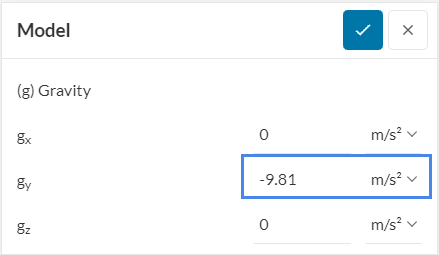
Select the Model tree element to specify the gravitational acceleration.

• Please set ‘9.81’ \(m/s²\) in the negative Y direction

2.2 Material

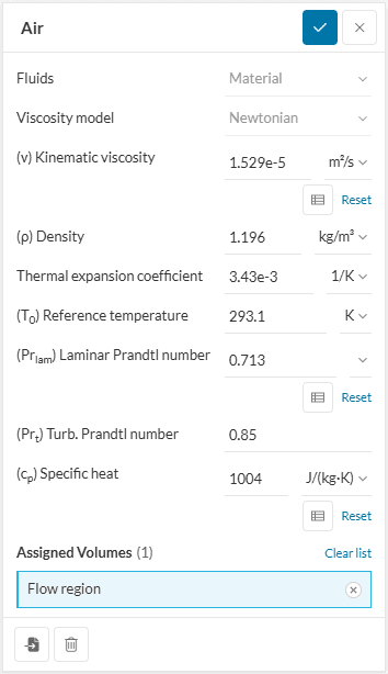
Next, we have to define the fluid inside our car, which will be air. We will use the standard air material from the SimScale library. To define and assign a material, please click on ‘+’ next to Materials. Doing so, the SimScale material library will pop up:

1. Select ‘Air’ from the materials library.
2. Click ‘Apply’.

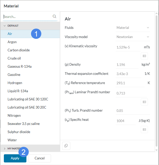
As there is only one flow region, it is automatically assigned. Accept the selection with the checkmark.

Since we do not simulate any heat transfer through solid materials the Solid material element will be left empty.

2.3 Boundary Conditions

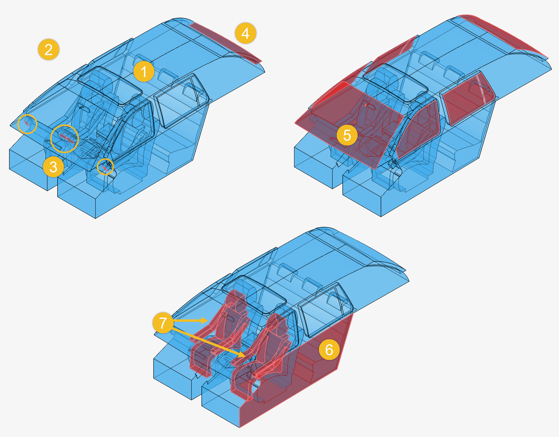
Now we will use the boundary conditions presented in Figure 8 to set these up according to the faces. Here we will also use the saved selections from the beginning of the tutorial for a faster setup.

A. Flow Inlet

At first, the boundary condition for the right inlet is created. After that, you can create the boundary conditions for the other inlets accordingly. These boundary conditions define from where air can enter the inside of the car. The setup is chosen in a way that we could switch between different vent settings like a closed vent on the right side. But for this case, we will assume that all vents are opened.

A flow velocity inlet boundary condition is created according to Figure 11 for the right inlet:

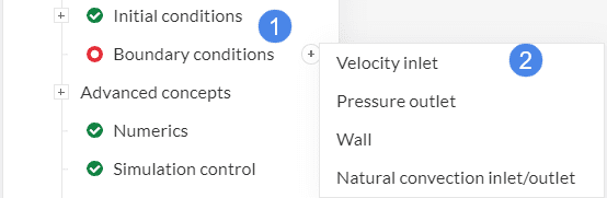
After hitting the ‘+’ button next to Boundary conditions, a drop-down menu will pop up where different types of boundary conditions can be chosen from. Select ‘Velocity inlet’ from the list.

Now the setup for the velocity inlet boundary condition will pop up.

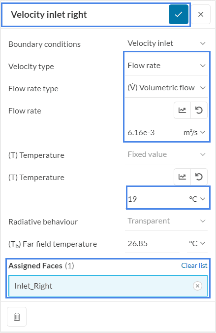
Please modify the following:

• Set a Volumetric flow rate of ‘0.00616’ \(m³/s\),
• Rename the Boundary to Velocity inlet right
• Temperature of ’19’ \(°C\)
• Assign the Inlet_Right saved selection as the face

You can find the Inlet_Right under the predefined saved selection on the right side of the Workbench.

In order to complete the inlet definitions repeat this process for the left, center, and top inlet with the volumetric flow rates given in table 1:

Boundary	Volumetric Flow rate \([m³/s]\)
Left	0.00616
Center	0.00616
Top	0.021

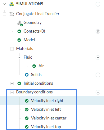
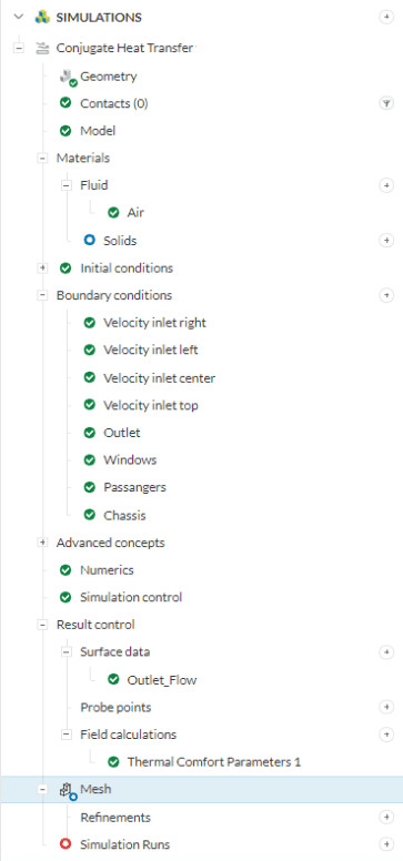
Now your Simulation tree should look like this, with all inlets defined and saved selections assigned:

B. Pressure Outlet

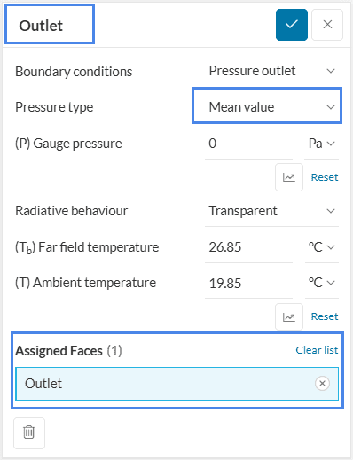
For the flow outlet boundary condition, follow the same procedure, but select ‘Pressure outlet’. Leave all values as default and assign the Outlet saved selection, as shown in the image. This will allow the air to exit the car freely through the face at the back of the car.

C. Windows

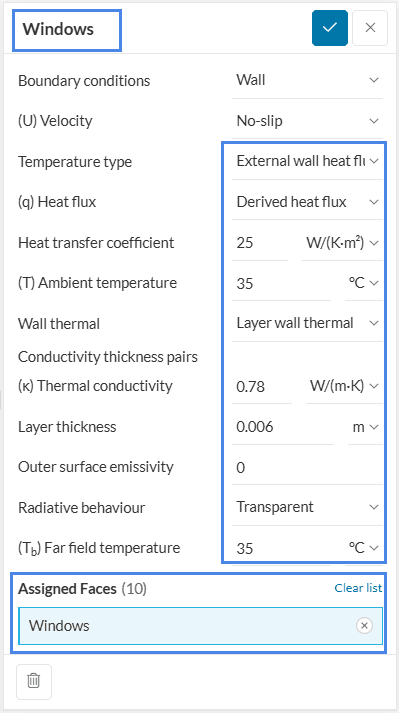
For the windows, we will have to define the radiative heat emitted. Therefore a wall boundary condition is used with a layer wall thermal model, convection to the exterior temperature, and an external radiation source to model sunlight.

Create a ‘Wall’ boundary condition and assign the Windows saved selection. Set up the parameters as shown in Figure 15:

D. Passengers

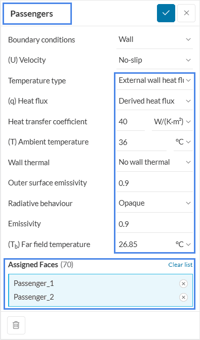
For the occupants, a wall boundary condition is also used, this time with a heat flux power source to model the metabolic heat generation rate. Create a ‘Wall’ boundary condition and assign the Passenger_1 and Passenger_2 saved selection. Continue with the setup with the parameters as shown in Figure 16:

E. Chassis

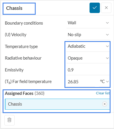
For the Chassis, a wall boundary condition is used, with adiabatic thermal behavior, since we assume that the car is perfectly insulated. Create a ‘Wall’ boundary condition and assign the Chassis set. Set up the parameters as shown in Figure 17:

2.6 Numerics & Simulation Control

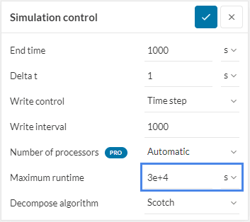
Since the mesh will contain around 5. Mio Cells we have to adjust the maximum runtime of the simulation. For that, we adjust the maximum runtime and give it a value of 30000 \(s\).

• Expand Simulation Control item and
• Set the Maximum runtime to ‘30000 \(s\)’

2.7 Result Control Items

Result control items are used to retrieve specific computations from the numerical solver. By using them, we can have a look at specific variables at specific regions by querying the computation and output of our quantities of interest. We will use this to determine how much the air heats up when passing through the car, by measuring the temperature at the outlet of the car.

A. Outlet Analysis

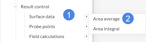
In order to measure the average outlet temperature a result control item is used. It’s created as shown in Figure 18:

1. Expand Result control and click the ‘+’ icon next to Surface data,
2. Select ‘Area average’

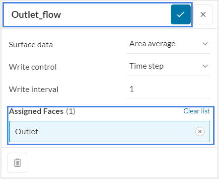
Assign the Outlet set and check that the setup coincides with Figure 19:

B. Thermal Comfort Parameter

To analyze the thermal comfort of the passengers a thermal comfort result control is defined.

Thermal Comfort Parameters

Thermal comfort parameters are also queried in the result control items, under Field calculations. Create the thermal comfort result control as shown in Figure 20 :

1. Click the ‘+’ button next to Field calculations and Select ‘Thermal Comfort Parameters’.
2. Set up the parameters as shown in Figure 20:
   • the Clothing coefficient is ‘0.5’,
   • the Metabolic rate is ‘1.0’,
   • the Relative air humidity is ‘65 %’.

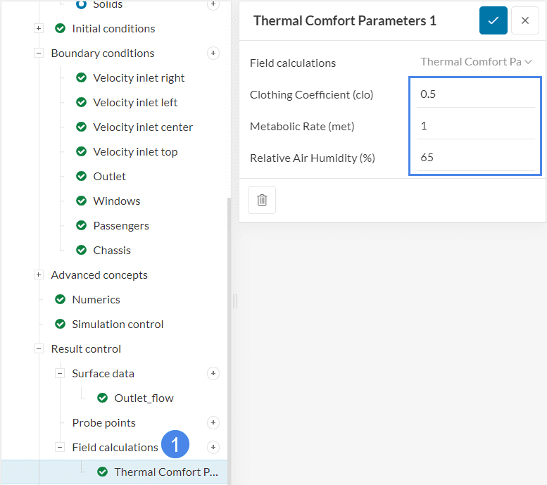
A description of the computed quantities and resulting fields can be found on this SimScale documentation page.

3. Mesh

For this tutorial, we will use standard meshing. Since we have already set up all the boundary conditions and assigned all faces of the Car_Internal_Volume geometry, we can use the automatic boundary layer, and the physics-based meshing feature. With that, we just have to change the Fineness to ‘6’.

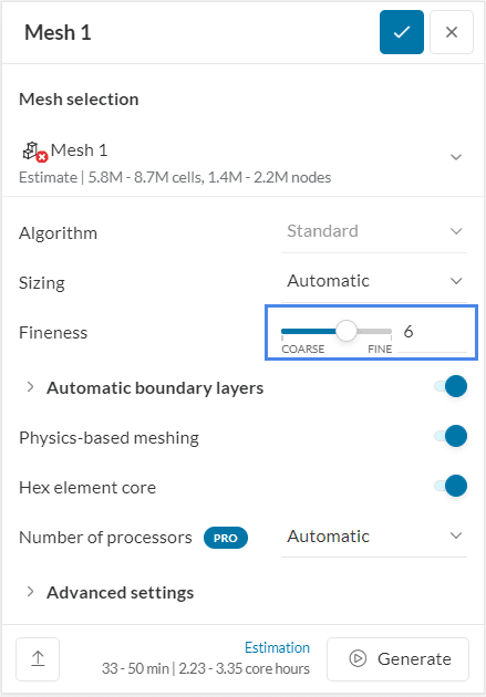
Don’t generate the mesh yet. The solver automatically performs it as we start the simulation.

4. Start the Simulation

Now that the simulation setup is complete, a new ‘Simulation Run’ can be created to perform the computation. In Figure 23, the whole tree setup is shown, and the item to create the simulation run is highlighted:

In the pop-up window, press ‘Start’ to immediately begin the simulation run. If the software predicts a higher duration of simulation and exceeds maximum runtime you can choose to ignore it or go back to simulation control settings and increase the maximum runtime value.

The computation takes around five hours to complete. If you can’t wait to see the results, at the end of the article there is a link to the completed version of the project.

5. Post-Processing

We will use the integrated post-processor to visualize the temperature and flow inside the Car Cabin and evaluate the thermal comfort by visualizing the Percentage Mean Vote (PMV).
Before starting to post-process the results, make sure that there are no predefined filters. You can delete existing filters at any time by clicking on the dustbin icon next to them. Furthermore, please ensure that you are at the last timestep of your simulation by sliding the Iterations selector all the way to the right. Lastly, hide the Flow region in the MESH dialog by clicking on the ‘eye’ icon.

5.1 Temperature

There are several methods to analyze the temperature within the car cabin, we will use both analytic and optical approaches.

A. Analyze the outlet Temperature

Before visualizing the temperature and analyzing it optically we can have a look at the average outlet temperature. For this, we go to the Area averages section > Area average 1, which is our outlet. Now we can select the temperature \([T]\) and see what the exit air temperature is.

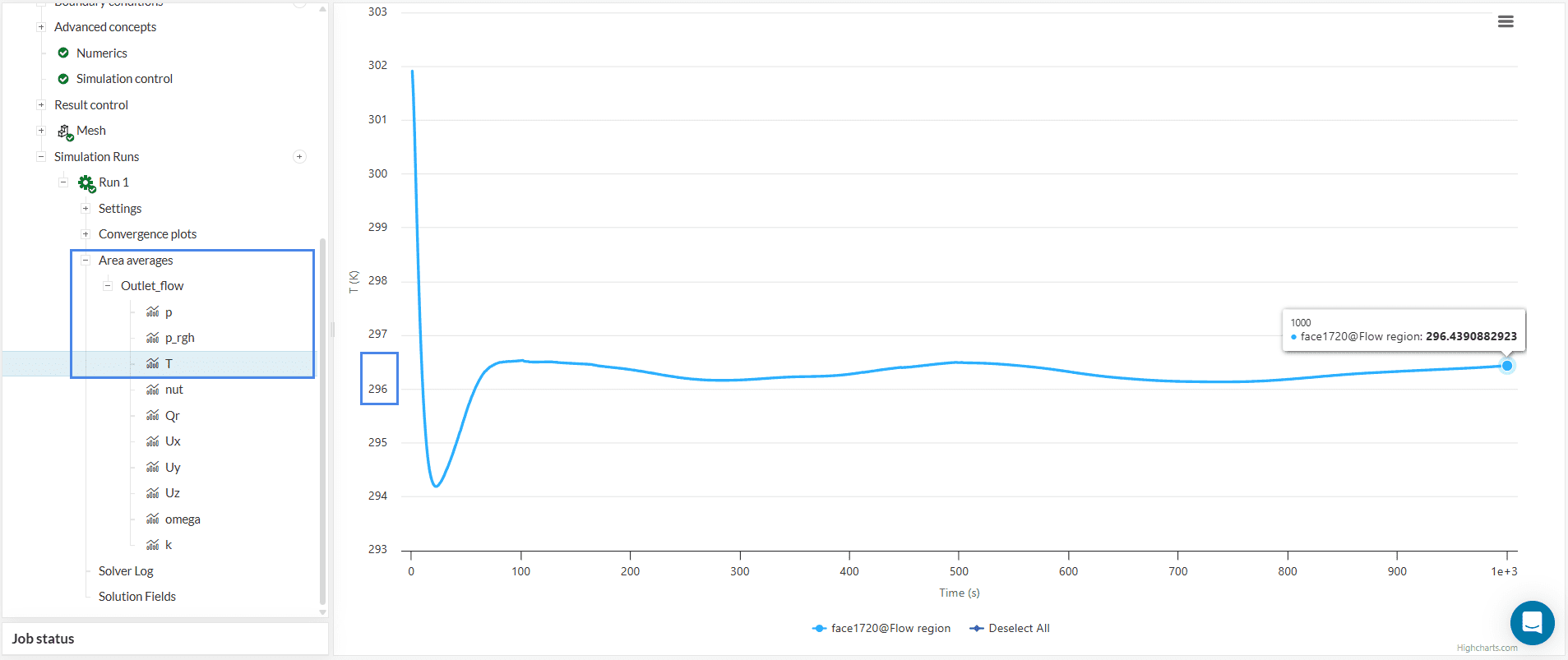
We see that the temperature has flattened out at 299 \(K\) ( ~27 \(°C\)). This means that the temperature has increased from the inlet to the outlet by 8 \(K\) in comparison to the inlet temperature, which we set to 19 \(°C\)

B. Visualization of the Surface Temperature

Next, we will visualize the temperature on the surfaces of the car. For that select ‘Temperature’ as the coloring for the parts. Change the units of temperature to Celsius by clicking the units in the legend and selecting ‘\(°C\)’ and changing the maximum temperature visualized to ’40’ \(°C\) and minimum to ’19’ \(°C\).

To have better look inside the car hide the roof and windows by selecting the faces and right-clicking on your mouse to select ‘Hide selection’.

The temperature distribution inside the car can be seen in Figure 25:

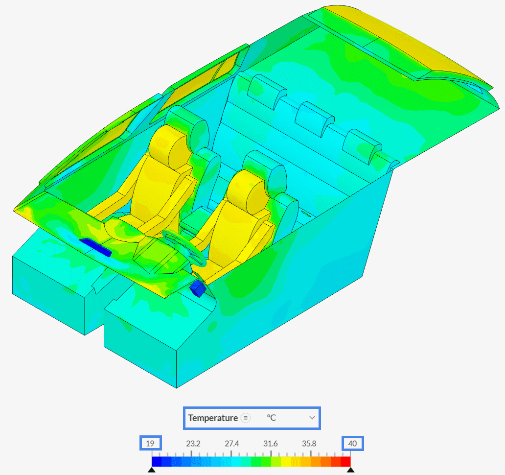
We can see how the windows are heated up by the radiation of the sun and the ambient temperature and how the passengers emit heat. Notice how the front windows are cooled by the cold airflow through the vent at the right, directing the hot air from the surface of the window to the back of the car.

5.2 Predicted Mean Vote

Next, we will have a look at the predicted mean vote for the passengers. For this, we will use the existing cutting plane. Change the y coordinate of the plane to ‘0.95’ \(m\) and the normal orientation to ‘Y’, so that we can analyze the thermal comfort at chest height.

To display the predicted mean vote change the coloring of the plane to ‘Predicted Mean Vote’. For a better visibility, we change the opacity of the plane to ‘0.7 ‘ and the Parts Color Coloring to a solid white color.

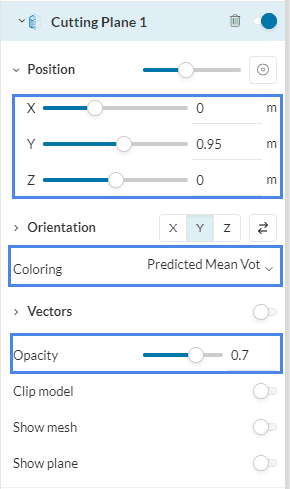
To clearly see the range of interests change the minimum scalar to ‘-2’ and the maximum to ‘2’. With that, we can clearly see the range in which the thermal comfort parameters are within the limits. The results are as follows:

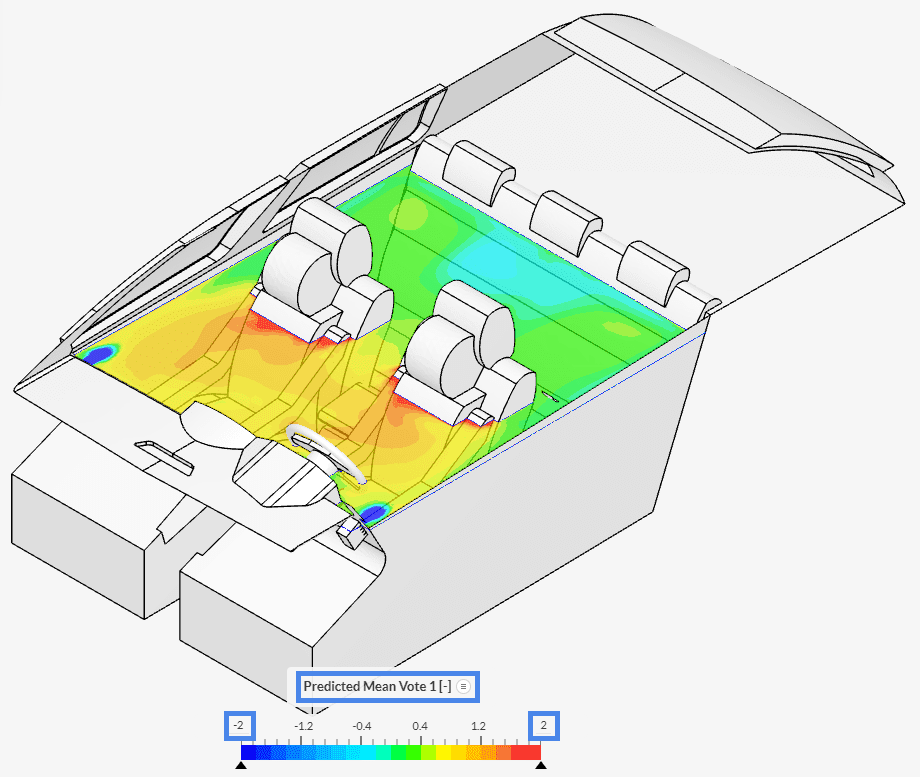
We see that in general, the predicted mean vote values are within the limits for this height. You can adjust the Y value for the position of the plane to see different areas like ‘1.1’ \(m\) for the head of the passengers.

5.3 Flow analysis

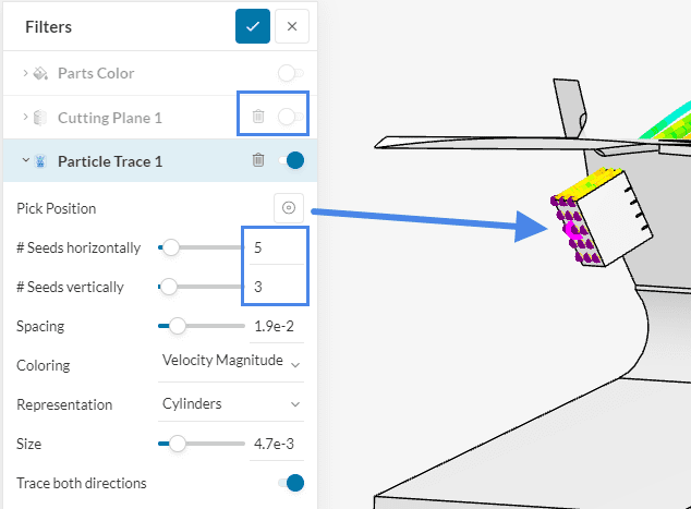
At last, we want to visualize the flow through the car cabin. For that, we will use Particle traces since this gives us a three-dimensional visualization of the flow through the car. Create a new particle trace by clicking on the ‘Particle trace’ icon.

Hide the cutting plane by using the toggle switch and then set the values according to the image below. For the position pick the center of the right inlet face. With that, we can follow the flow from the inlet to the outlet. If you are interested in other sections of the car you can always set the point to a different position.

Repeat the steps for the left inlet and one of the center inlets. You now have three-particle trace sets set up and the result should look like this.

We recognize that with the current setup most of the air from the ducts just passes the passengers. This cools down the air within the car without having the passengers sit in the flow stream directly.

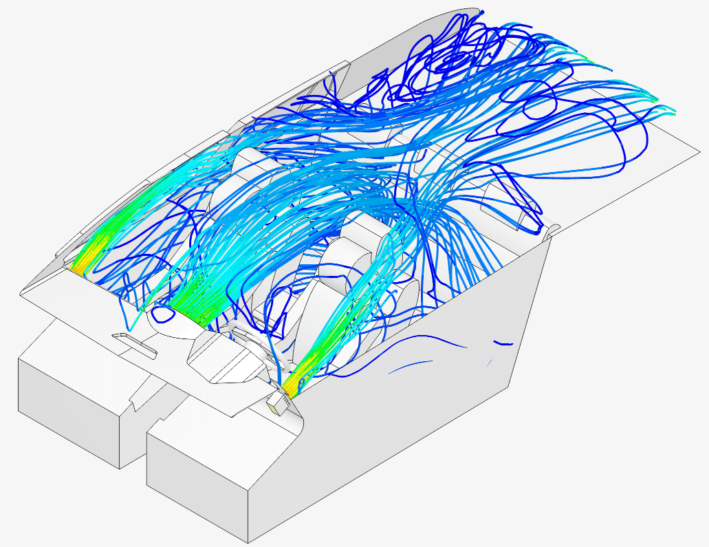
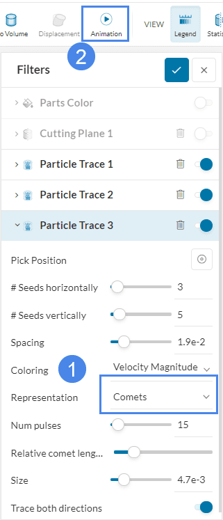
To create an animation of the particle traces change the particle representation to ‘Comets‘ and create a new animation filter by selecting the animation Icon. We select ‘Comets‘ for this step to not fill the car with the lines of the particle traces and be able to better follow a single particle through the car.

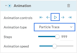
In the animation control panel, change the Animation type to ‘Particle Trace ‘ and start/stop the animation with the ‘play/pause button.

The results of the animation should look like this and we can follow a set of particles on its way through the car and for example analyze the turbulent flow behind the driver’s seat.

Analyze and explore your results with the SimScale post-processor. Have a look at our post-processing guide to learn how to use the post-processor.

Congratulations! You finished the tutorial!

Last updated: November 21st, 2023