Tutorial: Enclosure Snap Fit

With the following tutorial, you learn how to set up a nonlinear structural simulation. The case at hand is the snap-fit closing process of a plastic enclosure, as typically employed to house electronic devices.

We are following the typical SimScale workflow:

1. Preparing the CAD model for the simulation.
2. Setting up the simulation.
3. Creating the mesh.
4. Run the simulation and analyze the results.

1. Prepare the CAD Model and Select the Analysis Type

Firstly, click the button below. It will copy the tutorial project containing the geometry of the snap-fit into your Workbench. You can see the geometry of the enclosure in the 3D viewer, and interact with it using typical mouse gestures for rotating, panning, and zooming.

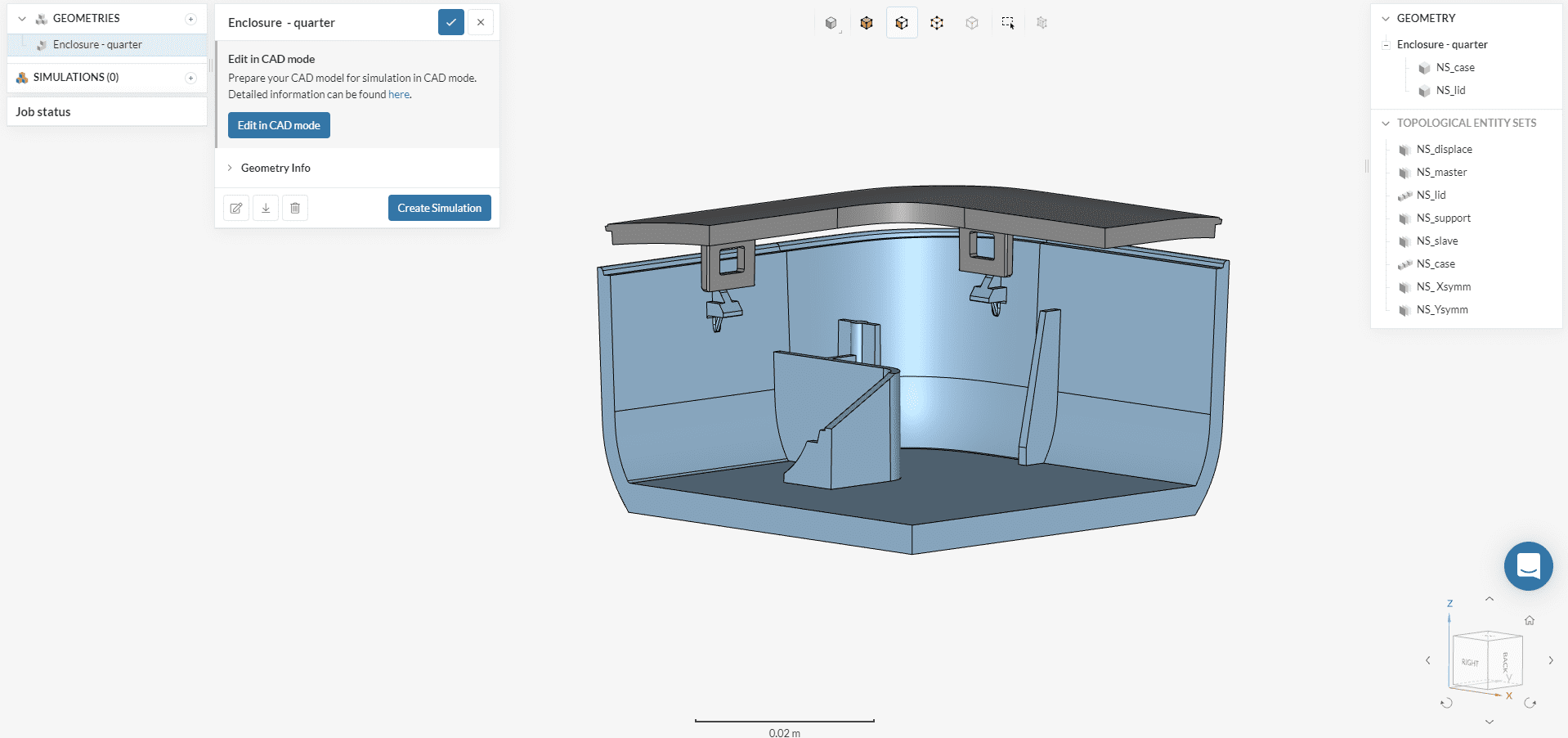
You can see that some Topological Entity Sets are already pre-defined for you on the right-hand panel in the Workbench. These will speed up our setup process.

1.1 Create the Simulation

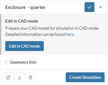
To create a new simulation using the enclosure geometry, first, make sure that the “Enclosure – quarter” geometry is selected (the geometry details window is shown as seen in Figure 2). Click on the ‘Create Simulation’ button.

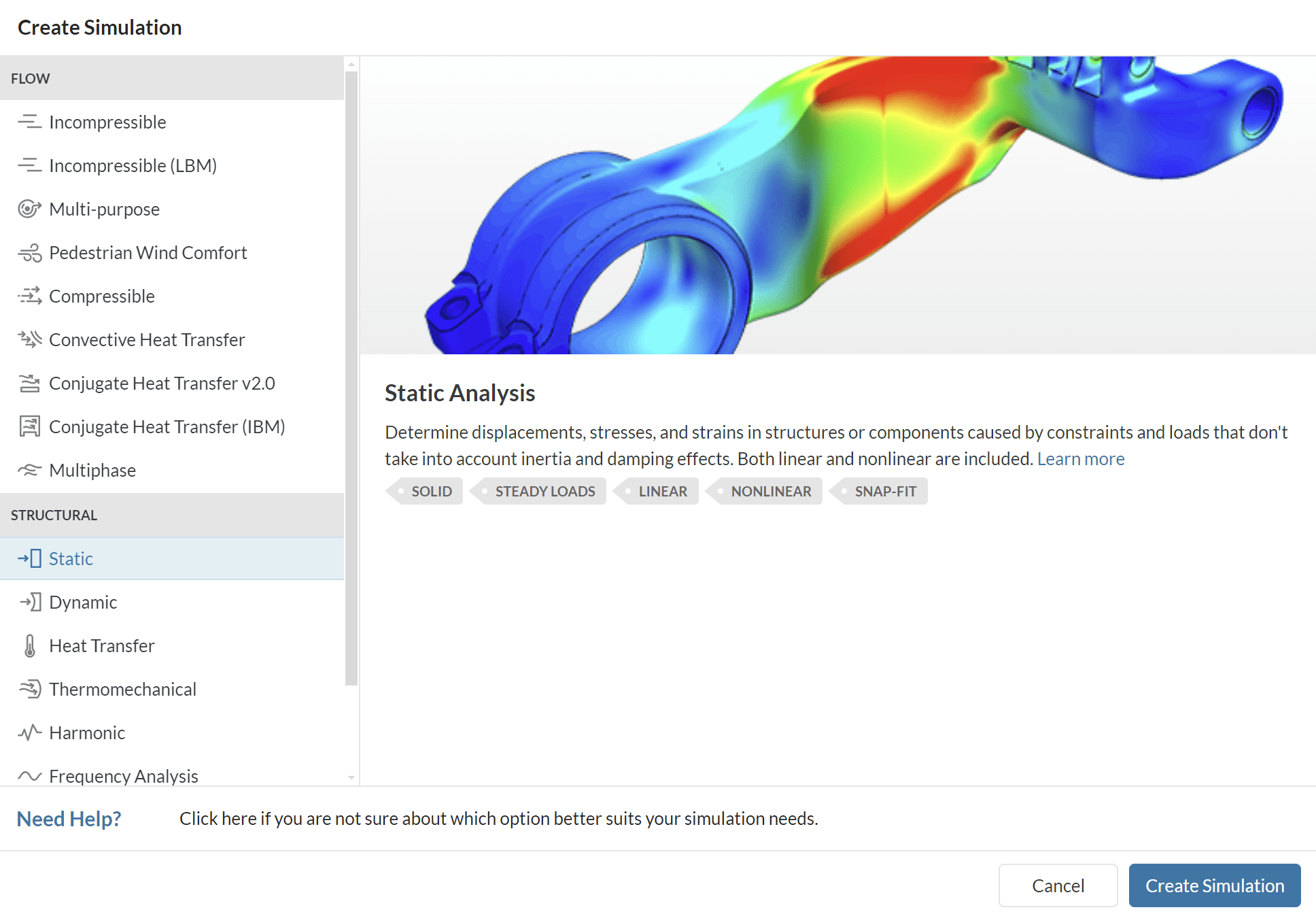
From the list of available simulation types, select ‘Static’, then click ‘Create Simulation’ at the bottom of the window.

A new simulation tree item is automatically created in the left panel of the Workbench. This tree contains all the parameters and settings required to define the simulation model. You can see items with a green check (setup is complete), a red circle (setup is mandatory), or a blue circle (setup is optional). We will walk down the lane in this tutorial to have all of them complete.

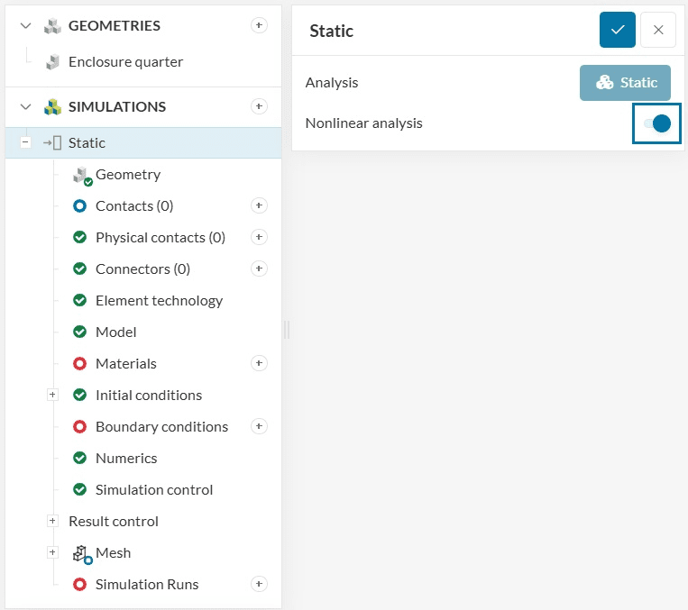
As the ‘Static’ simulation tree item is selected, the general settings panel is shown. The first action we will take is in this panel, by toggling on the ‘Nonlinear analysis’. This will enable the simulation to handle the large displacement of the lid, as well as the physical contacts on the tabs. Before you set the toggle, your simulation tree will look a little bit differently than the one shown in the picture above.

2. Physical Contact

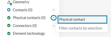
First, let’s create the physical contact. This will enable the mechanical interaction between the two parts, so the collisions and the snap fits are properly captured. To create a new physical contact definition, click the ‘+’ button next to Physical contacts (0), and select ‘Physical contact’ from the list.

Set up the physical contact in the panel as follows:

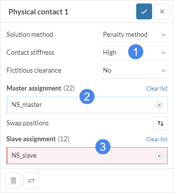
1. Set the contact stiffness to ‘High’.
2. For the Master assignment, select the ‘NS_master’ topological entity set from the right-hand panel.
3. For the Slave assignment, select the ‘NS_slave’ topological entity set from the panel.

3. Materials

To create a new material definition, click the ‘+’ icon next to Materials in the simulation tree. The materials library window is displayed, where you can select a material model from the default library, or from your custom materials library.

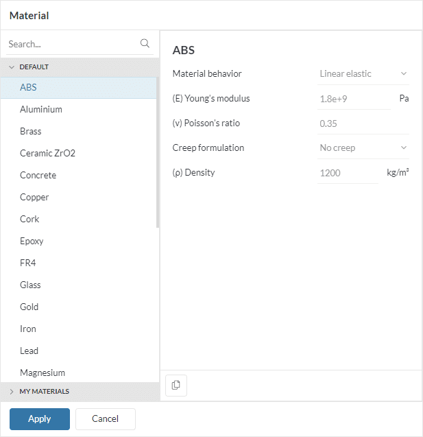
You can select any item from the list and click ‘Apply’, as we will fully customize it as follows:

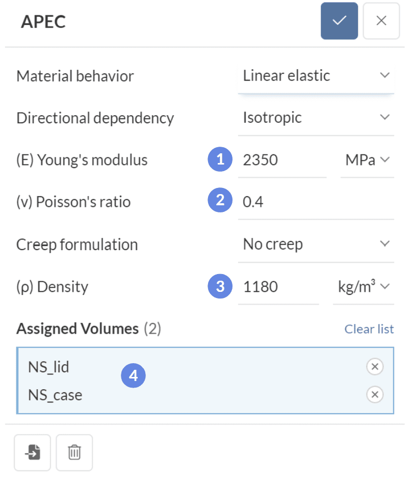
1. Set Young’s modulus to 2350 \(MPa\). Don’t forget to change the units!
2. Set the Poisson’s ratio to 0.4
3. Set the Density to 1180 \(kg/m^3\)
4. Assign the volumes ‘NS_lid‘ and ‘NS_case‘ from the topological entity sets panel.

4. Boundary Conditions

For the boundary conditions, we will set up what is known as a displacement-driven simulation, with the lid moving toward the fixed case. As the snap-fit model is quarterly symmetric, we need to include symmetry boundary conditions.

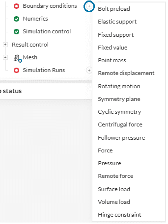
To create a boundary condition, simply click the ‘+’ icon next to Boundary conditions, then select from the list the type of boundary condition that you will apply, as shown below:

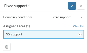
4.1 Fixed Support

Create a Fixed support boundary condition, then just assign the ‘NS_support‘ set for it. This will completely fix the displacements in the base of the case.

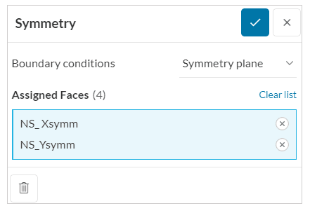
4.2 Symmetry

To specify the symmetry condition on the two symmetry planes in the model we will use a Symmetry plane boundary condition. Create the condition and assign the ‘NS_Xsymm’ and ‘NS_Ysymm’ sets to it:

4.3 Lid Movement

For the lid closing movement, we will use a Fixed value boundary condition. Set the \(d_x\) and \(d_y\) displacements as unconstrained, while the \(d_z\) displacement is set to -0.005 \(m\). Finally, assign the set named ‘NS_displace’.

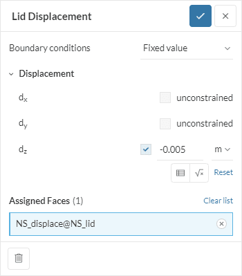
Notice how SimScale automatically detects the nonzero displacement and ramps up the value with time to ensure the numerical convergence of the simulation. This means that there is no need to enter a table of formulas for the displacement ramp.

5. Result Control

Measuring the force curve for the snap-fit process is one of the target results for our simulation. To obtain such a curve, one can use a Result control item. More specifically, an Area calculation over the same face with imposed displacement is able to retrieve the Sum of the Reaction Force.

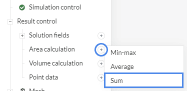
Let’s create one such item as shown by using the ‘+’ icon next to Area calculation, under Result control, then selecting a ‘Sum’ item from the list:

A new pop-up is shown, please set it up as shown:

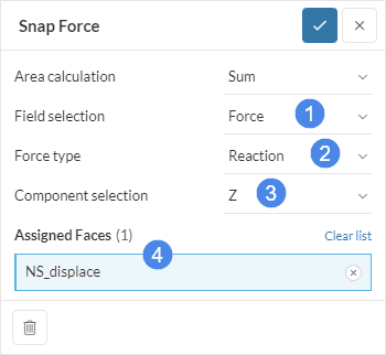
1. Select the ‘Force’ field
2. For the Force type, select ‘Reaction‘
3. For the component, set ‘Z’, which coincides with the direction of the movement and the specified displacement for the lid
4. For the assignment, select the ‘NS_displace’ set, which is the same used for the lid displacement boundary condition.

6. Simulation Run

As you can notice, there are no more red circles in our simulation tree. This means we can launch the computation! For this, let’s create a new simulation run by using the ‘+’ icon next to ‘Simulation Runs’.

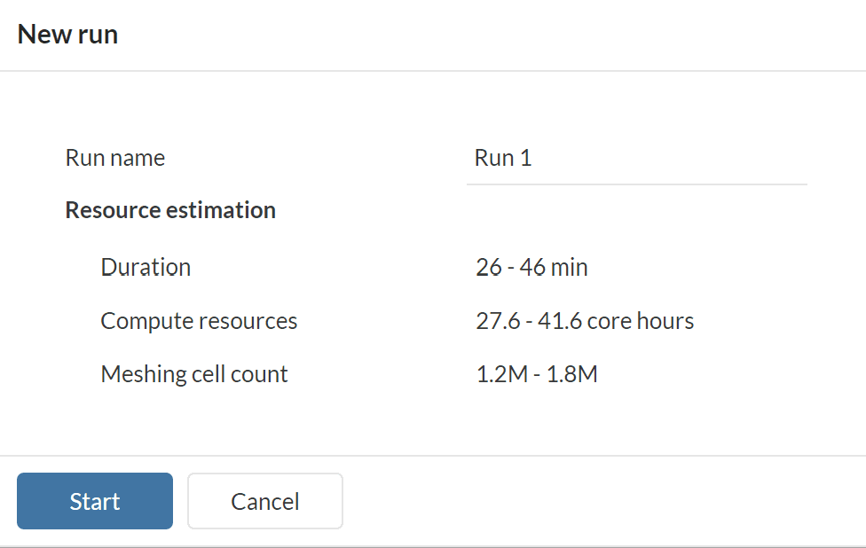
In the pop-up window, you might receive a couple of yellow warnings. We can safely ignore them and click ‘Run anyway’, then ‘Start’ on the New run window. The computation is launched and an email notification will be sent when it finishes.

7. Simulation Results

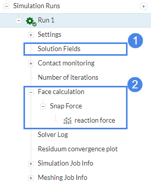
To visualize the results of the simulation you can use the online postprocessor. You can access it by selecting the ‘Solution Fields’ item under the successful simulation run (marked 1 in the figure):

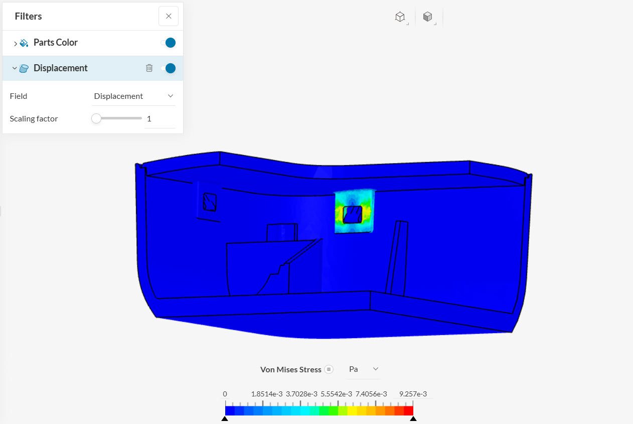
The online postprocessor is opened, showing the results. By default, the snap-fit model is colored by von Mises stress and deformed by a Displacement filter. You can find the currently visualized step on the right-hand panel (the simulated pseudo-times are labeled from 0 to 1).

You can cycle back and forth through the closing process by using the arrows in the STEPS panel at the right hand of the Workbench. But, here we will create an animation:

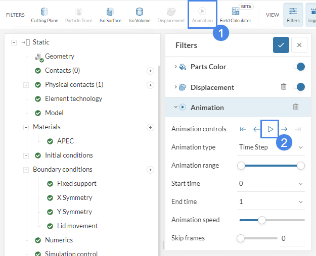
1. Select the Animation filter from the top bar.
2. In the Animation filter panel, click the play button.

After loading you should be able to see the displacement process:

Finally, let’s check our snap force curve. Select ‘Face calculation – Snap Force – reaction force’ as shown in figure 17. The plot view is displayed showing the force curve:

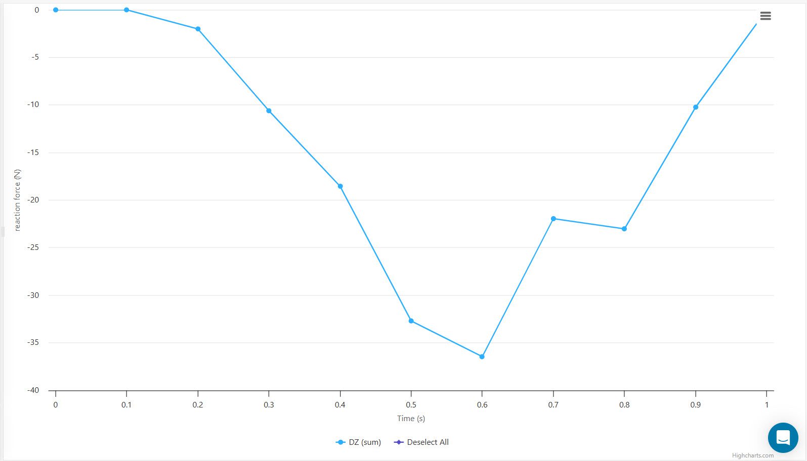
We can see that a maximum downward force of around 36 \(N\) is required to snap the lid onto the enclosure. We have simulated a quarter of the model thus in reality a total force of 144 \(N\) is required to mount the lid. This corresponds roughly to a double-handed pushing action and is suitable for this type of product.

Congratulations! You just finished your nonlinear structural simulation in SimScale!

For more tutorials, please visit the following page:

SimScale Tutorials and User Guides

Last updated: October 29th, 2024