Documentation
This article is inspired by the original Bending of an Aluminium Pipe tutorial—which uses SimScale’s Standard FEA Static analysis type—and provides a step-by-step guide for performing a nonlinear structural simulation of an aluminium pipe bending process using the ‘Nonlinear Mechanical (Marc)’ analysis type. The objective is to analyze the deformation and stress distribution that develop in the pipe during bending, including nonlinear effects such as material plasticity, physical contact, and large deformations.
This tutorial explains how to:
The tutorial follows the standard SimScale workflow:
Select the button below to copy the tutorial project, including the aluminium pipe geometry, into your workbench.
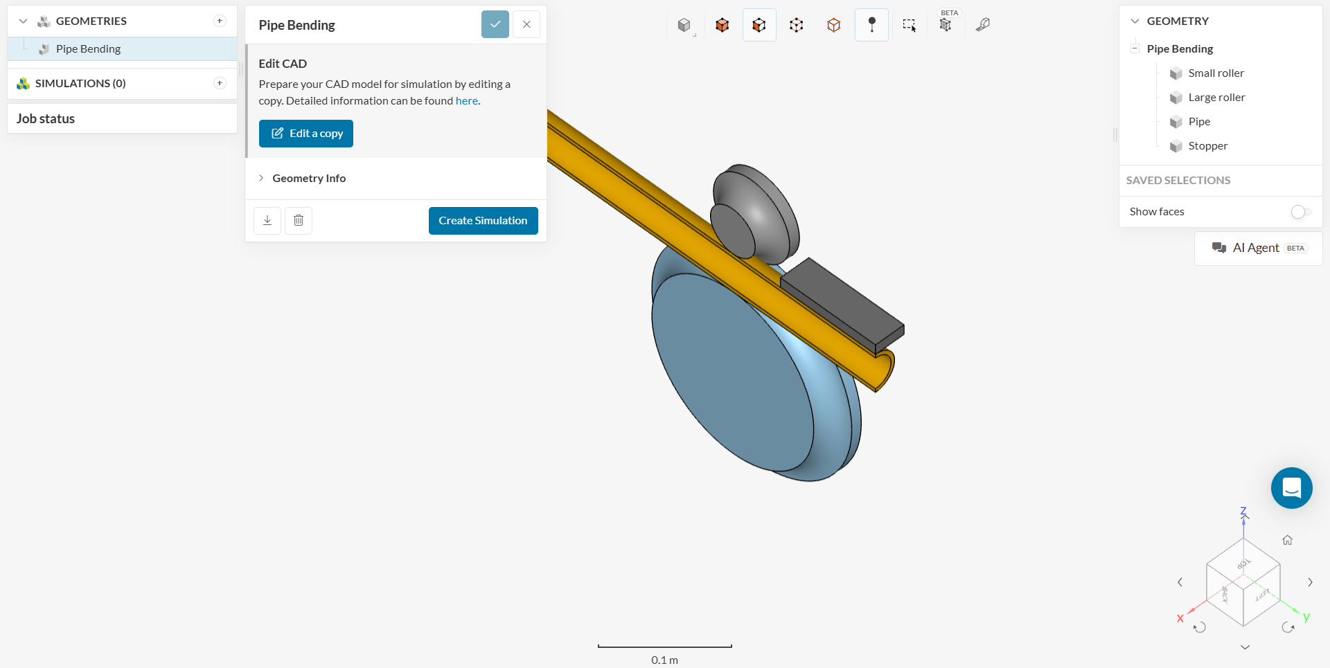
The image below shows the interface after importing the tutorial project.
If you are using your own CAD model, follow these instructions:
All solid geometry should be free of any interference, intersecting surfaces, and small edges. Fix these issues in CAD before importing the geometry into the SimScale platform. Refer to the CAD preparation guide for more details.
Before starting the simulation setup, verify the following:
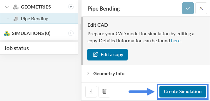
To begin the simulation setup, select the ‘Create Simulation’ button located in the geometry dialog box. This action opens the simulation creation panel where analysis types are selected.
The simulation type selection panel appears, allowing the selection of the desired analysis type.
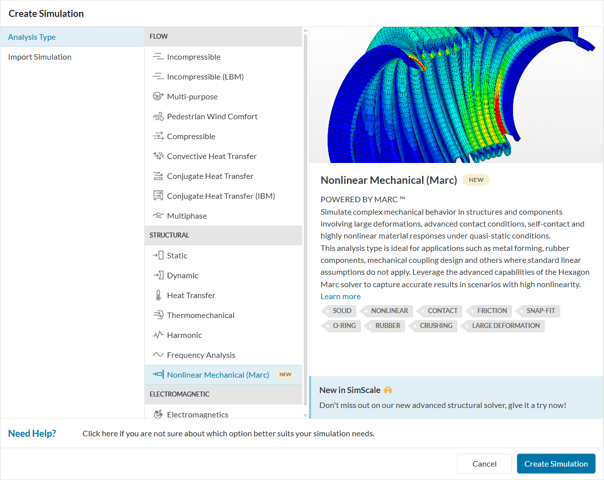
Select ‘Nonlinear Mechanical (Marc)’ as the analysis type and click the ‘Create Simulation’ button to proceed.
Studies using the Nonlinear Mechanical (Marc) analysis type are nonlinear, accounting for nonlinear contact relationships and material properties. This analysis differs from a Dynamic analysis, which accounts for inertial forces.
This tutorial simulates the forming process of an aluminium pipe using a hydraulic bending machine to evaluate the mechanical stress and strain induced in the components. Figure 5 illustrates the model components and the process:
The following modeling techniques are used to simulate the process:
With the analysis type selected, SimScale automatically detects several Glued contacts:
The contact between the pipe and the stopper is kept as ‘Glued’ to ensure no relative motion between contact nodes. The other two relationships are manually updated to ‘Touching’ contacts to capture real interactions, such as separation and contact changes.
Refer to this documentation page for more information about Marc contacts.
SimScale automatically detects touching faces or edges and assigns ‘Glued’ contacts by default. In this case, three contacts are identified:
Only the contact between the pipe and the stopper (‘Glued 3’) is required. Redefine the other two as ‘Touching’ contacts:
Under the Connectors node, establish a remote point connection between the largest circular face of the small roller and a remote point. This defines a rotation using the ‘Point displacement’ boundary condition later in the setup. Create a new point under the ‘Geometry primitives’ node in the simulation tree as presented in the figure below.
Follow the steps outlined in Figure … :
Navigate back to the ‘Connectors’ node and select the ‘+’ icon to generate a ‘Remote point connection’. Leave the ‘Behavior’ as ‘Rigid (RBE2)’, select the created point under ‘Point’, and select the largest face of the small roller. This action links the face and the point through rigid body elements.
What is the difference between RBE2 and RBE3 elements?
In FEA, RBE (Rigid Body Element) connects a remote point to a set of nodes. RBE2 creates an infinitely rigid link where the remote point governs the movement of the surface, preventing local deformation. RBE3 acts as an interpolation element that distributes loads or mass without adding stiffness, allowing the connected surface to deform naturally.
Retain the default settings and proceed to ‘Materials’.
This simulation assigns two different materials:
To create a new material, select the ‘+’ icon next to ‘Materials’ to open the materials library. Select the required material and click ‘Apply’ to create the material item:
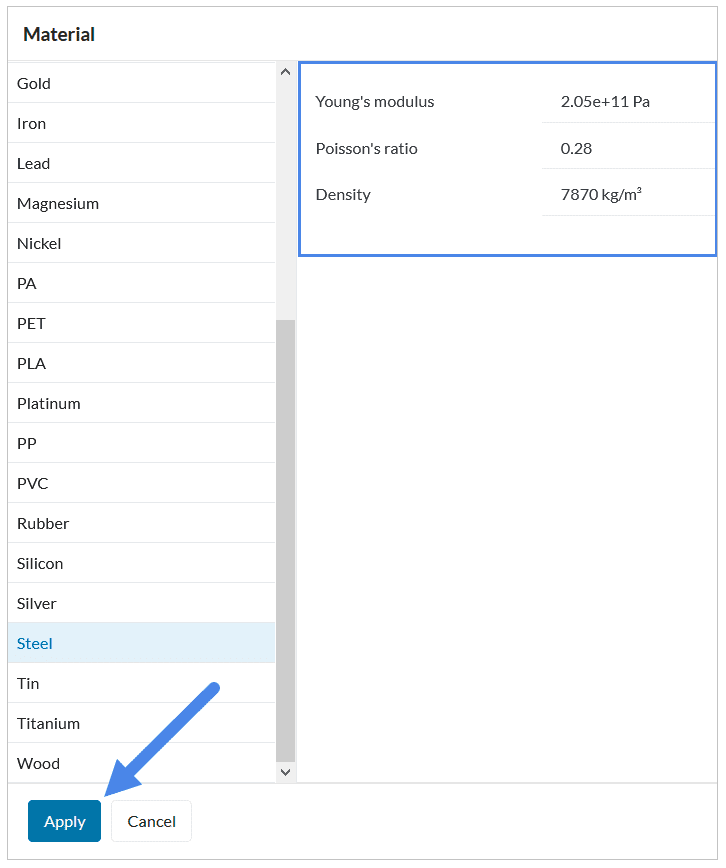
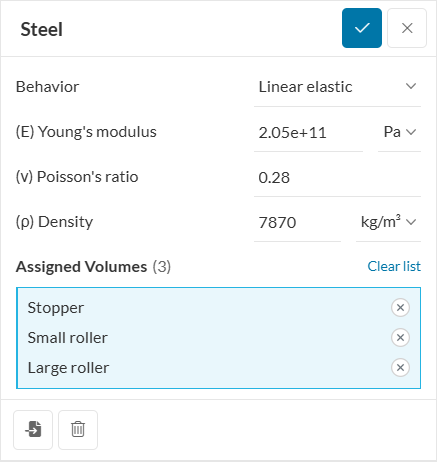
Create a ‘Steel’ material and assign it to the ‘Stopper’, ‘Small roller’, and ‘Large roller’. Other parameters remain at their default values:
Repeat the procedure for the pipe using ‘Aluminium’. The ‘pipe’ body is automatically selected as it is the only remaining body without a material assignment.
Figure 10 displays the true stress-plastic strain curve for the material. Switching the ‘Behavior’ to ‘Elastoplastic’ enables permanent deformation calculation.
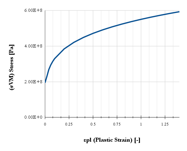
To model this nonlinear behavior, change the material ‘Behavior’ to ‘Elastoplastic’ and set the parameters as shown in Figure 13. The stress curve \( \sigma \) data is provided in the following steps.
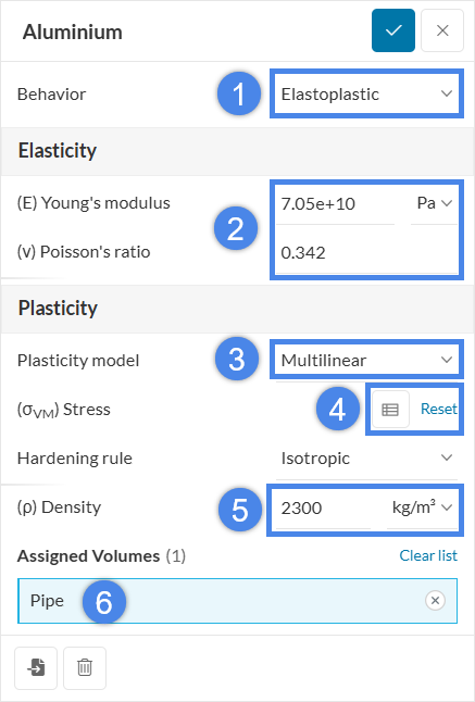
The solver requires the aluminium stress-strain curve shown in Figure 10 to predict deformation. Select the button below to download the material data CSV file:
Select the ‘Table input’ icon in the material window (highlighted in Figure 10). This action opens the ‘Specify value’ window:
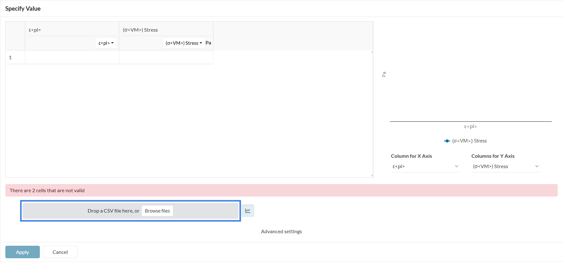
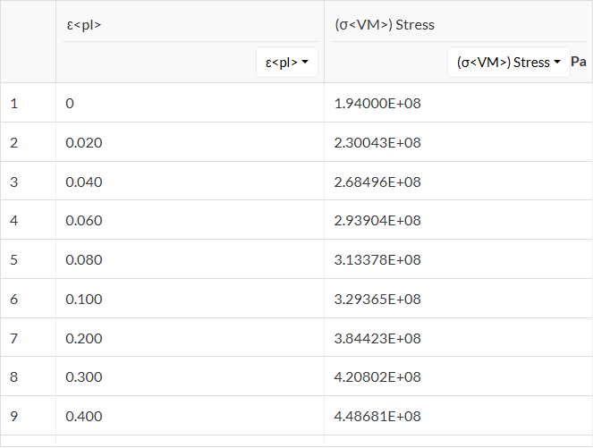
Select the ‘Browse files’ button to upload the CSV file. The data table populates as follows:
Click ‘Apply’ in the settings shown in Figure 15 to confirm the data, then select the ‘Check-mark’ icon to save the setup. This resolves the error message indicated in Figure 14.
Refer to Figure 6 for an overview of the physical setup to inspect the boundary conditions defined in this section.
To define a boundary condition, select the ‘+’ icon next to ‘Boundary conditions’ in the simulation tree and select the required type from the dropdown menu:
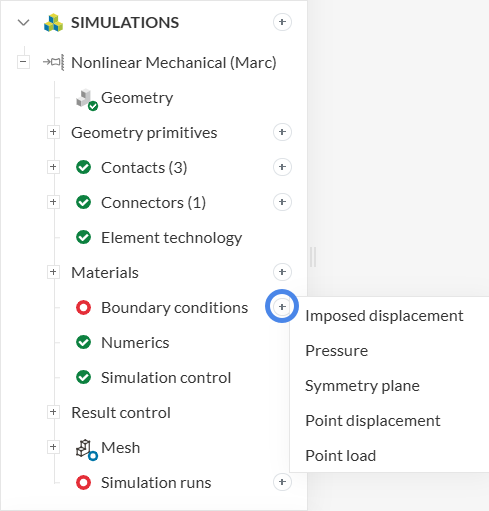
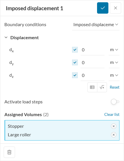
Define an ‘Imposed displacement’ boundary condition.
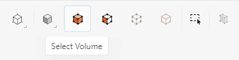
Face selection mode is active by default. To assign solid bodies, use the scene tree to switch to volume selection mode:
Assign the boundary condition to the ‘Large roller’ and ‘Stopper’ bodies. As shown in Figure 5, these must be constrained in X, Y, and Z (set to \(0\)).
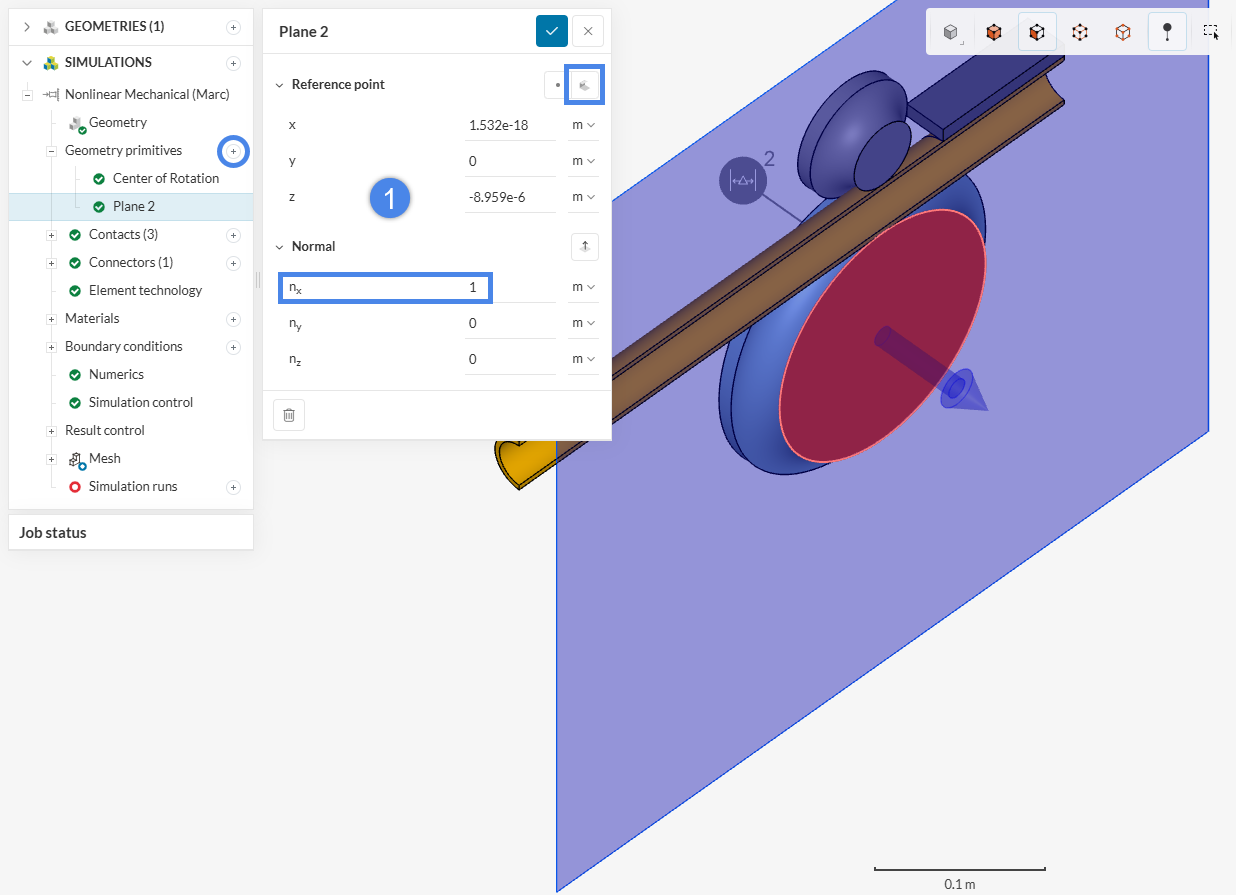
The geometry includes only half of the pipe and components to optimize computational resources. To apply a ‘Symmetry plane’ condition, create a ‘Plane’ under the ‘Geometry primitives’ node by selecting a reference point at the surface of a symmetric face and setting the normal (e.g., \(n_x = 1\)).
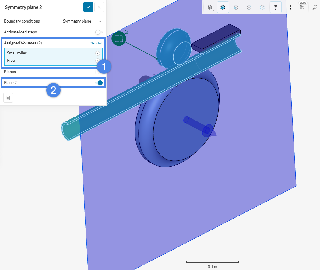
Define a ‘Symmetry Plane’ boundary condition, assign the ‘Small roller’ and ‘Pipe’, and activate the plane created previously under ‘Planes’. The ‘Large roller’ and ‘Stopper’ are excluded as they are already fixed.
How does a symmetry plane work in Marc?
In Nonlinear Mechanical (Marc), a symmetry plane acts as a rigid plate constraining planar nodes and serving as a barrier for contact interactions.
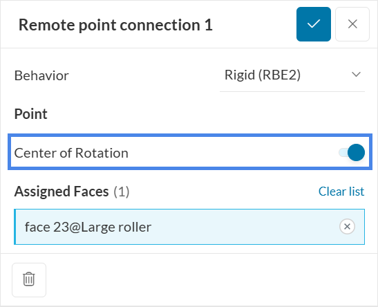
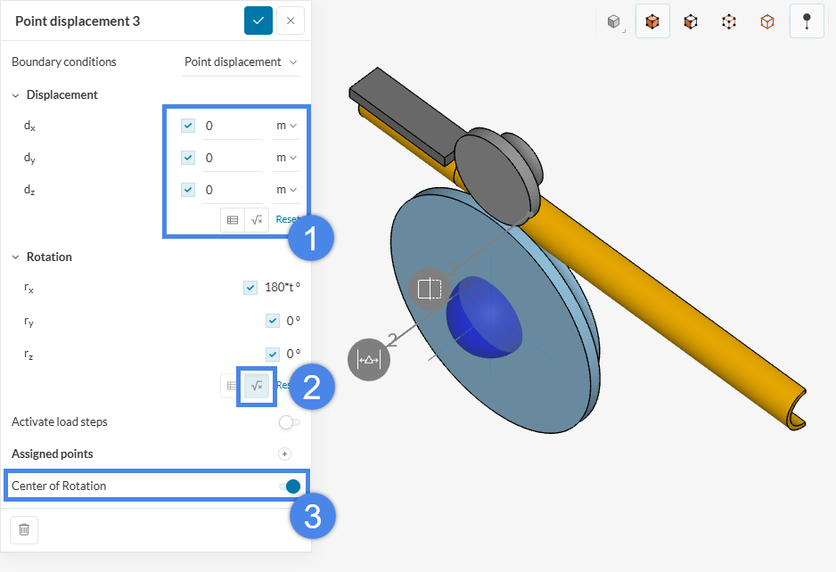
For the small roller, define a ‘Point displacement’ boundary condition. Fix the ‘Displacement’ values to prevent translation and select the Center of Rotation under ‘Assigned points’.
An equation defines the linear ramping of the angular motion in the \(r_x\) direction. Figure 19 illustrates the simulated motion from \(0^\circ\) to \(180^\circ\):
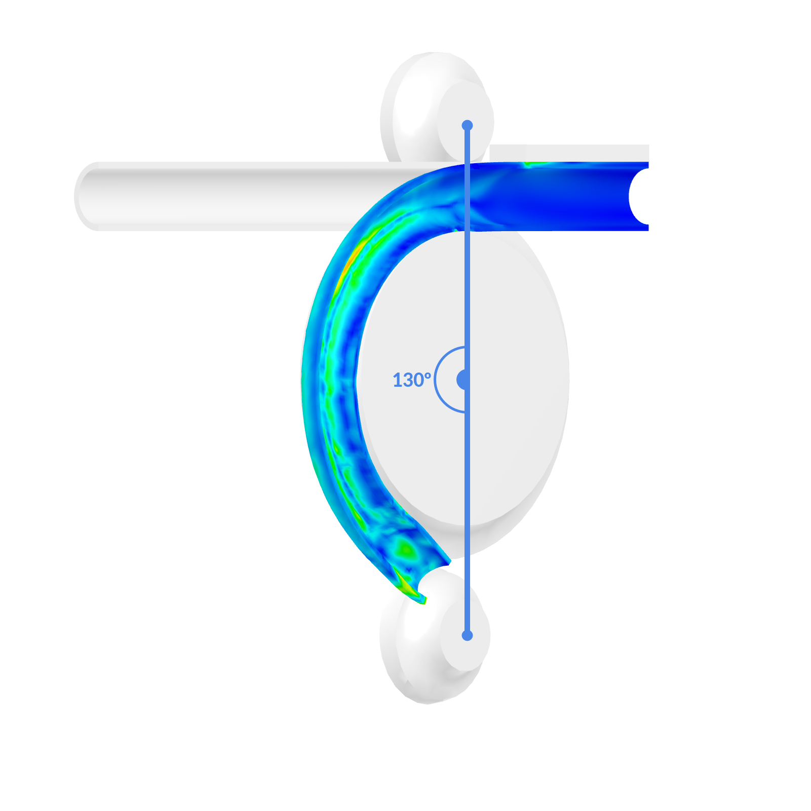
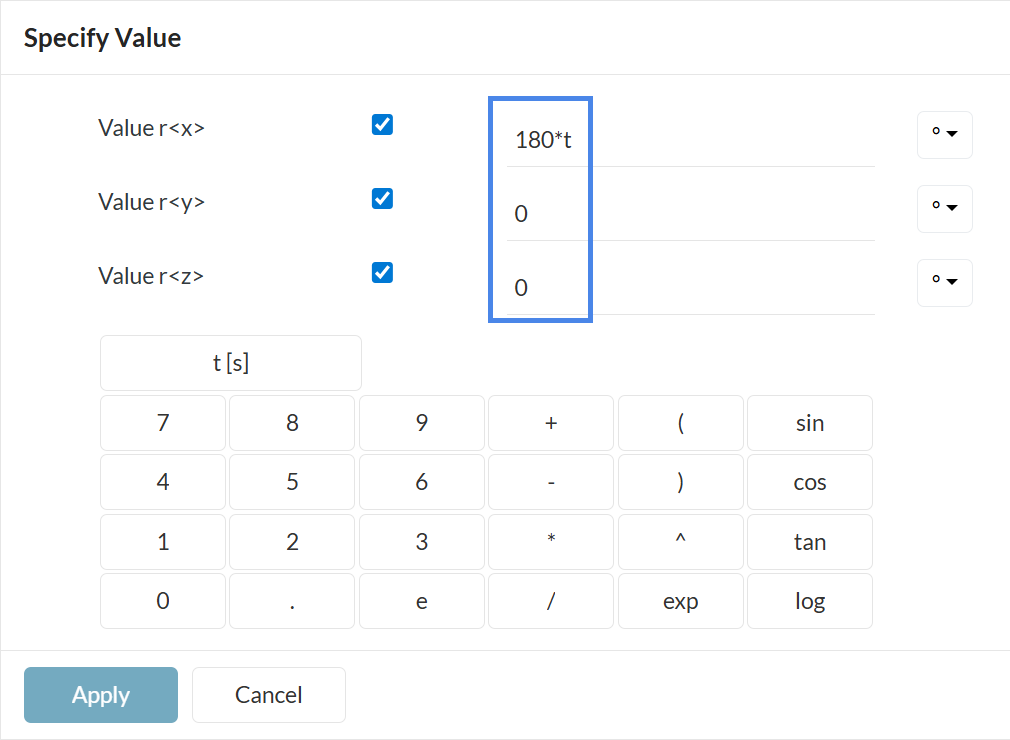
A positive \(180^\circ\) rotation is required. The corresponding equation is \( \phi(t) = 180 \times t \). Select the ‘Formula’ icon in the boundary condition settings (highlighted in Figure 18) to enter the formula shown in Figure 20.
Select ‘Apply’ and the ‘Check-mark’ icon to save the setup.
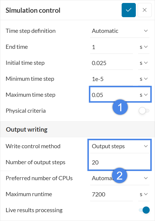
The ‘Numerics’ parameters control solver precision; retain the default settings. In ‘Simulation control’, set the ‘Maximum time step length’ to \(0.05\ s\), change the ‘Write control method’ to ‘Output steps’, and set the ‘Number of output steps’ to \(20\).
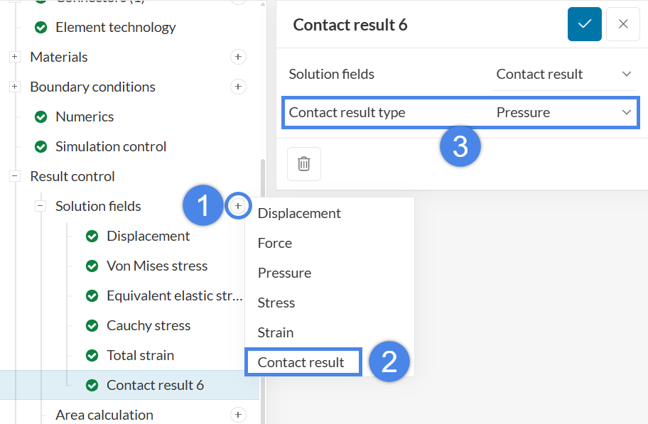
‘Result control’ defines the output fields. In addition to the defaults, a ‘Contact result’ field is required.
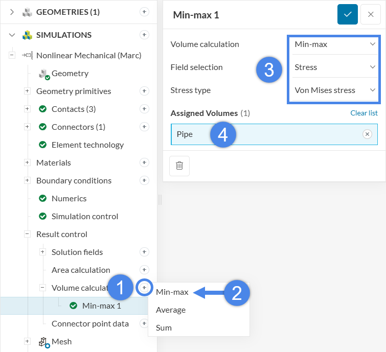
Volume calculations report field statistics over a part. Define a ‘Volume calculation – Min-max’ item for the ‘von Mises stress’ over the ‘Pipe’ as shown in Figure 24.
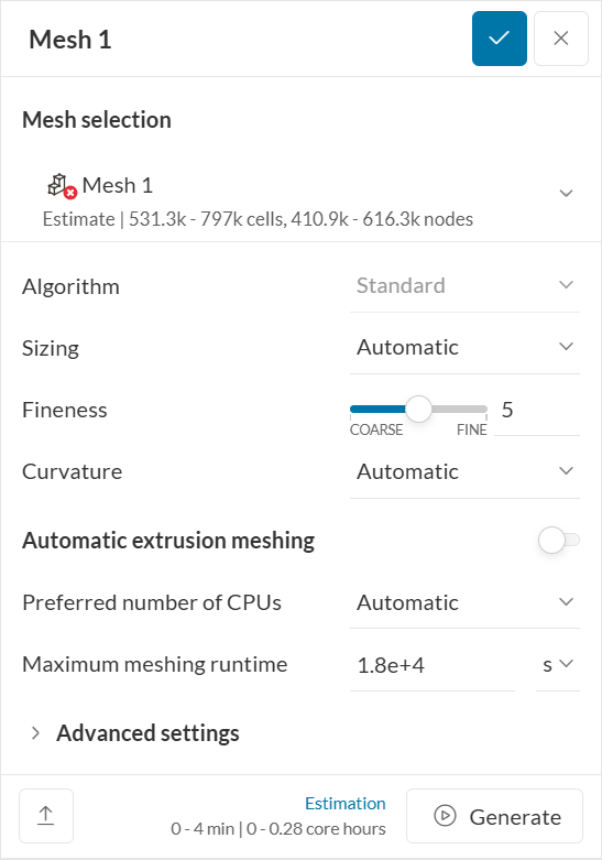
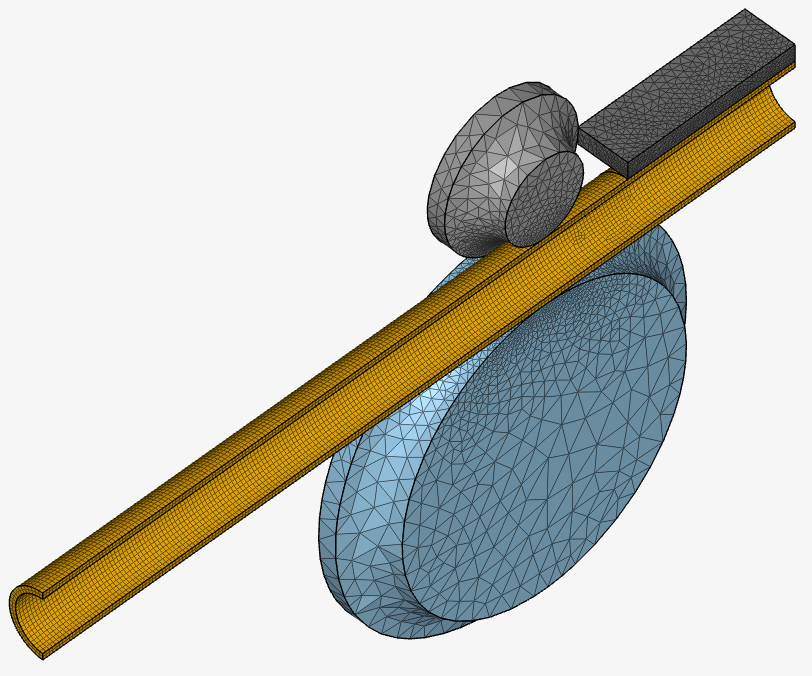
This tutorial uses the standard mesh algorithm with default general settings:
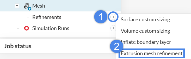
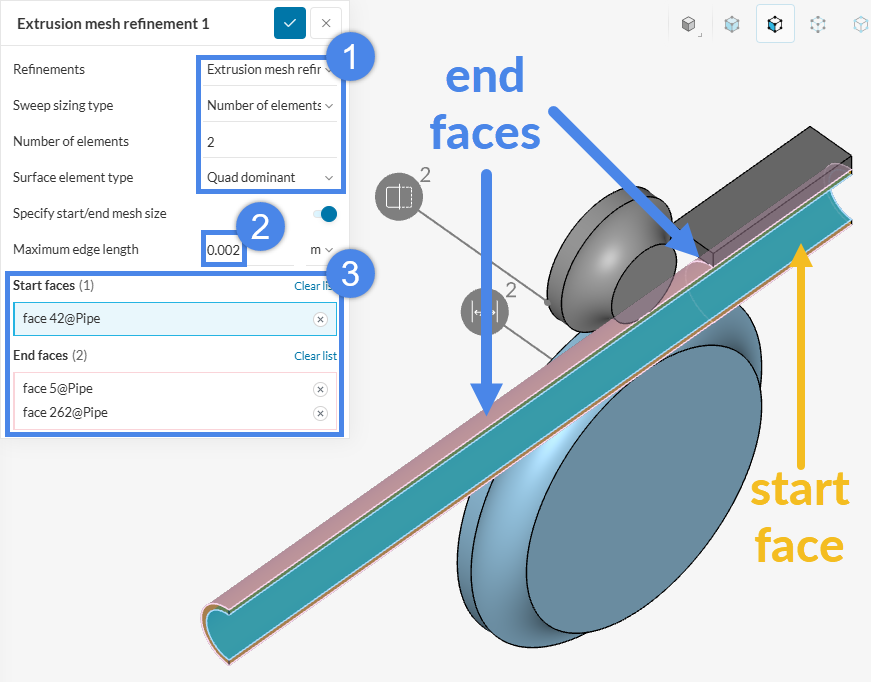
Apply local refinements to optimize resources. An ‘Extrusion mesh refinement’ improves the mesh in thin sections. Follow the steps in Figure 26 to define the refinement.
Assign the refinement to the pipe faces (Figure 27). Set ‘Sweep sizing type’ to ‘Number of elements along sweep’ at \(2\), use ‘Quad dominant’ as the ‘Surface element type’, and set a ‘Maximum edge length’ of \(4 \times 10^{-3}\ m\).
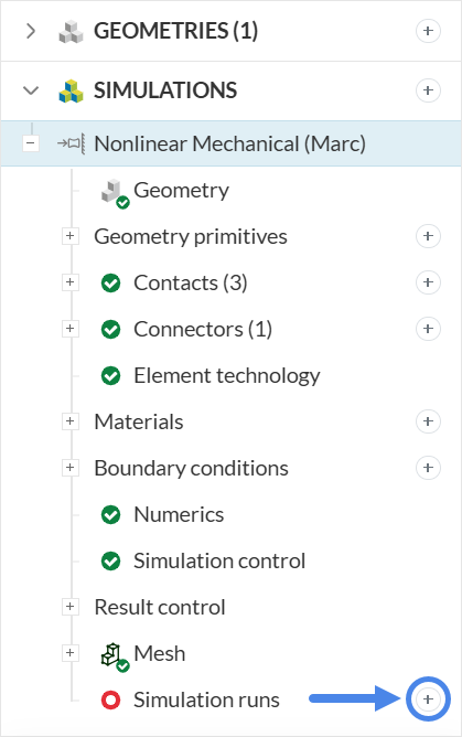
Create a new run by selecting the ‘+’ icon next to ‘Simulation Runs’:
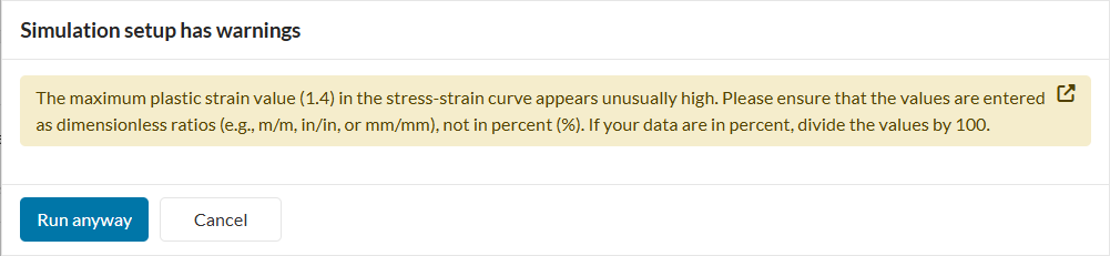
Important
When you create a simulation run, the following warning message will appear:
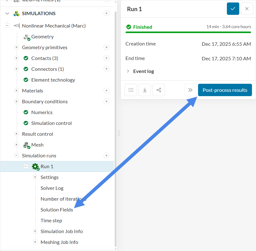
Once the run is successful, open the online post-processor using the ‘Solution Fields’ node or the ‘Post-process results’ button (Figure 31).
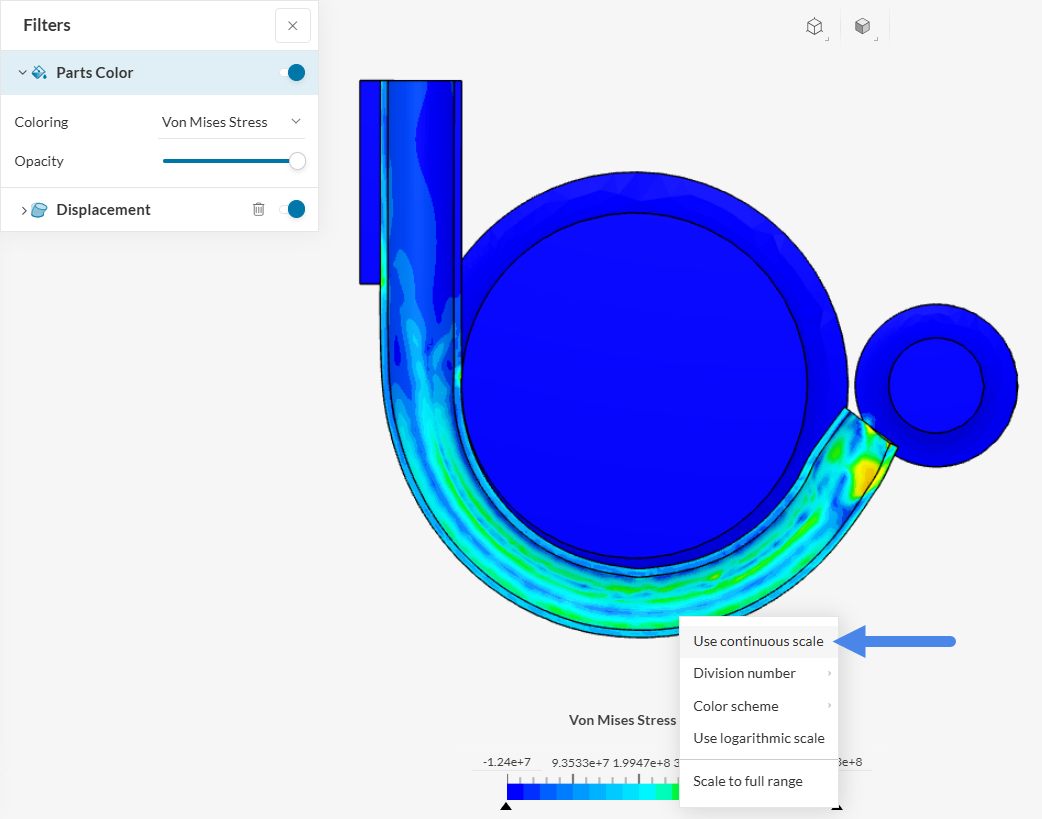
By default, ‘Displacement Magnitude’ is selected for ‘Coloring’ under ‘Parts Color’. Select ‘Von Mises Stress’ instead, right-click the legend and select ‘Use Continuous Scale’ to improve result visualization (Figure 32).
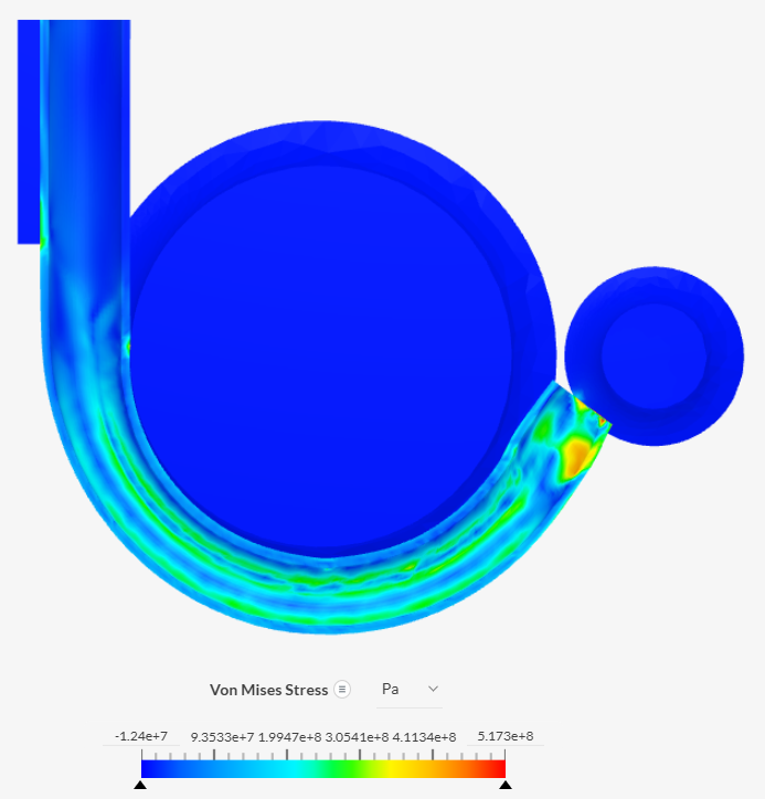
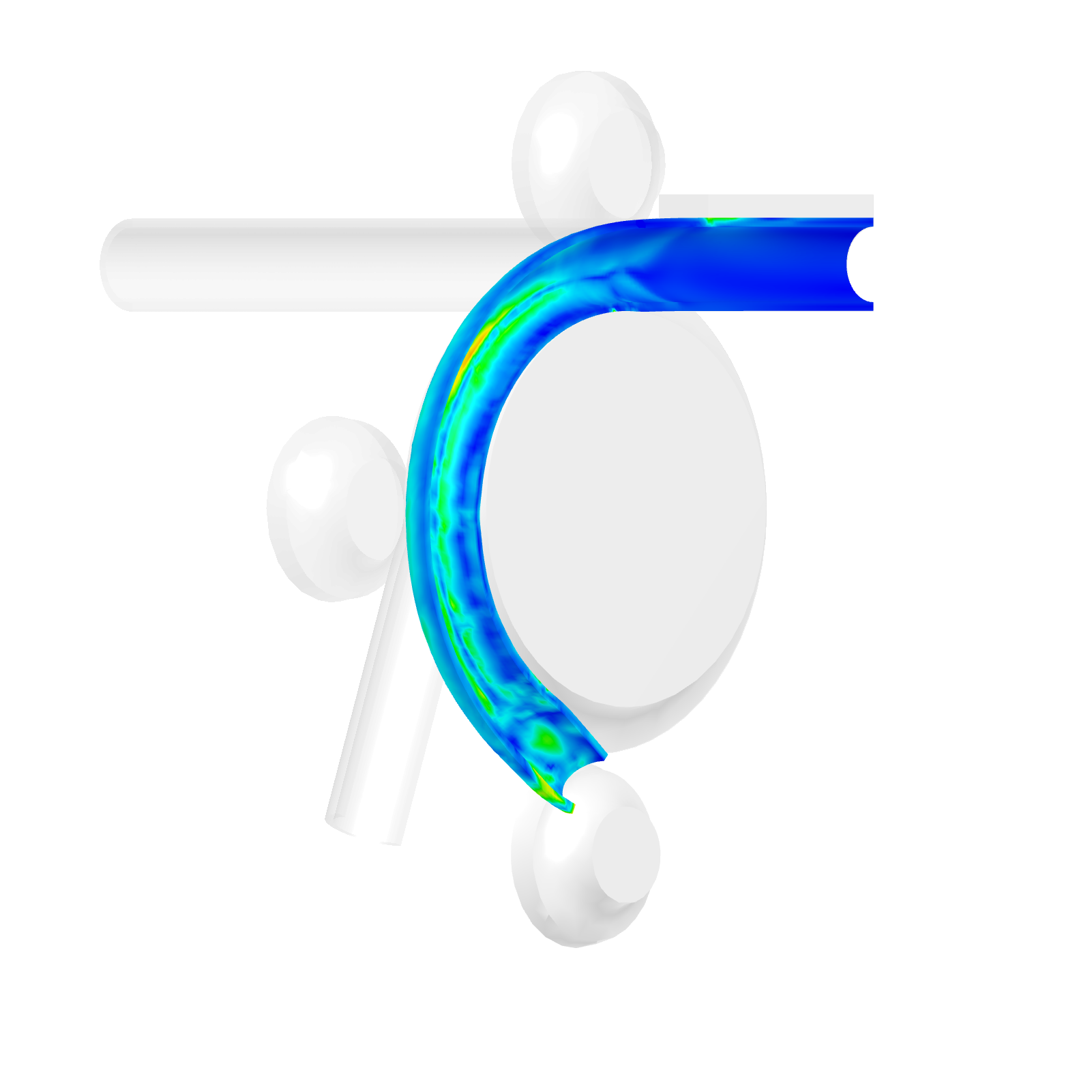
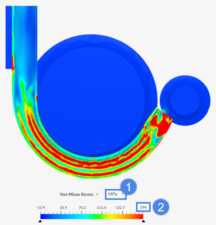
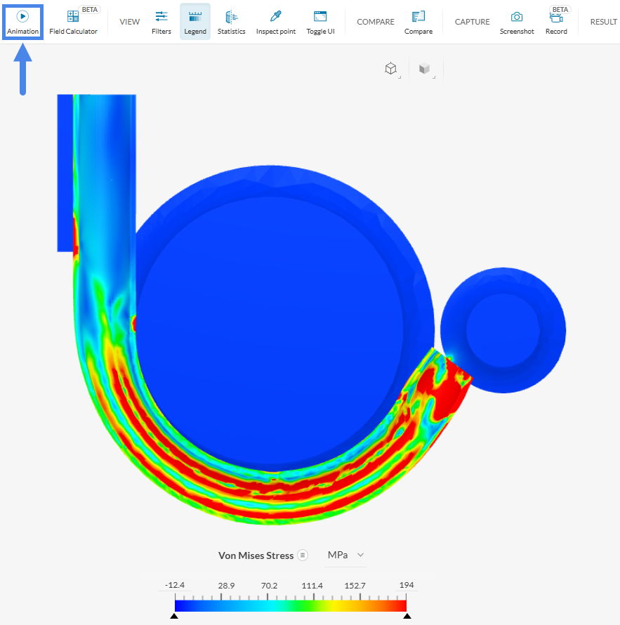
Inspect the ‘Von Mises Stress’ and update the units to \(MPa\) and the maximum scale to the yield stress of \(194\ MPa\) (Figure 34).
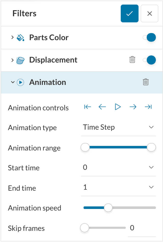
Create an ‘Animation’ filter as established for the ‘Displacement’ filter using the top bar (Figure 35).
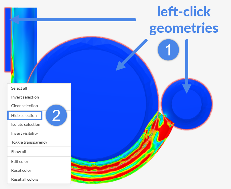
To inspect the stress distribution without obstruction, select the parts in the viewer, right-click, and select ‘Hide Selection’ (Figure 37).
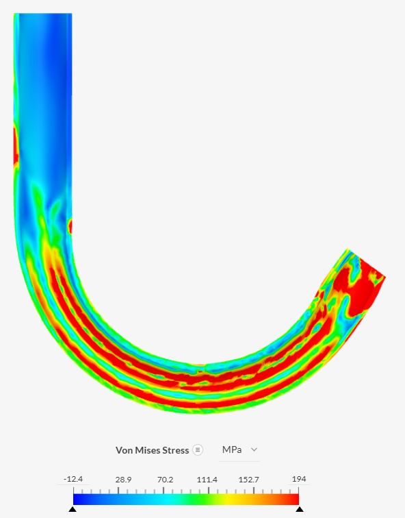
Inspect how parameters affect the results and explore different visualizations. For additional details, refer to the post-processing guide.
Congratulations! The tutorial is complete.
Note
If you have any questions or suggestions, please reach out via the forum or contact us directly at support@simscale.com.
Last updated: March 3rd, 2026
We appreciate and value your feedback.
Sign up for SimScale
and start simulating now