What is Laminar Flow?

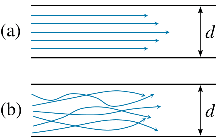
Fluid flows can be classified as laminar flow and turbulent flow. Laminar flow occurs when the fluid flows in infinitesimal parallel layers with no disruption between them. In laminar flows, fluid layers slide in parallel, with no eddies, swirls or currents normal to the flow.

This type of flow is also referred to as streamline flow because it is characterized by non-crossing streamlines (Figure 1). That means every fluid particle follows the same trajectory of its preceding particle. Laminar flow is common when the fluid is moving slowly, through a relatively small channel, and/or with high viscosity.

The laminar regime follows momentum diffusion, while momentum convection is less important. In more physical terms, it means that viscous forces are higher than inertial forces.

Schematic diagram of laminar and turbulent flow in a closed pipe — Figure 1: (a) Laminar flow in a closed pipe, (b) Turbulent flow in a closed pipe. The laminar region is smooth with less chaos because the turbulent flow has high momentum convection.

Join SimScale Today!

Laminar Flow vs Turbulent Flow

The distinction between laminar and turbulent regimes was first studied and theorized by Osborne Reynolds in the second half of the 19th century. His first publication$^{1}$ on this topic is considered a milestone in the study of fluid dynamics.

This work was based on the experiment used by Reynolds to show the transition from the laminar to the turbulent regime.

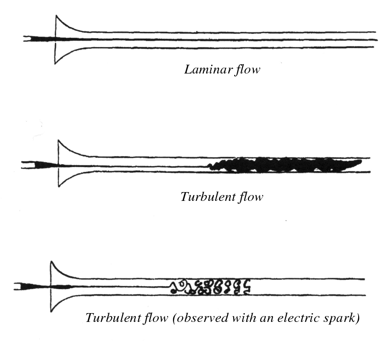
The experiment consisted of examining the behavior of water flow in a large glass pipe. In order to visualize the flow, Reynolds injected a small vein of dyed water into the flow and observed its behavior at different flow rates.

When the velocity was low, the dyed layer remained distinct throughout the entire length of the pipe.
When the velocity was increased, the vein broke up and diffused throughout the tube’s cross-section, as shown in Figure 2.

Thus, Reynolds demonstrated the existence of two different flow regimes, called laminar flow and turbulent flow, separated by a transition phase. He also identified a number of factors that affect the occurrence of this transition.

Reynolds' experiment showing the laminar, transition and the turbulent flow phases. — Figure 2: Reynolds’ experimental observation of the transition phase showing the streamlined dye gradually transitioning to eddies and swirls.

Reynolds Number

Reynolds number (Re) is a dimensionless number expressing the ratio between inertial and viscous forces. George Gabriel Stokes first introduced the concept in 1851, but Osborne Reynolds popularized it and proposed it as the parameter to identify the transition between laminar and turbulent flows. For that reason, the dimensionless number became Reynolds number, named by Arnold Sommerfeld after Osborne Reynolds in 1908$^2$.

Reynolds number is a macroscopic parameter of flow in its globality and is mathematically defined as:

$$ Re=\frac{\rho u d}{\mu} =\frac{ud}{\nu} \tag{1}$$

where:

$\rho$ is the density of the fluid
$u$ is the macroscopic velocity of the fluid
$d$ is the characteristic length (or hydraulic diameter)
$\mu$ is the dynamic viscosity of the fluid
$\nu$ is the kinematic viscosity of the fluid

Fluid Flows and Their Corresponding Reynolds Number Values

At low values of Reynolds number, the flow is laminar. When the Reynolds number exceeds a threshold value, semi-developed turbulence occurs in the flow. This regime is usually referred to as the “transition regime” and occurs for a specific range of the Reynolds number. Beyond that range, the flow becomes fully turbulent.

The mean value of Reynolds number in the transition regime is usually named “Critical Reynolds number”. It is the threshold between the laminar and the turbulent flow.

It is interesting to notice that the Reynolds number depends both on the material properties of the fluid and the geometrical properties of the application. This has two main consequences:

The Reynolds number describes the global behavior of flow, not its local behavior; in large domains, it is possible to have localized turbulent regions that do not extend to the whole domain. For this reason, it is important to understand the physics of the flow to determine the accurate domain of application and the characteristic length.
The Reynolds number is a property of the application. Different configurations of the same application may have different critical Reynolds numbers.

The following table shows the correspondence between the Reynolds number and the regime obtained in different problems.

Problem Configuration	Laminar regime	Transition regime	Turbulent Regime
Flow around a foil parallel to the main flow	$Re<5\cdot 10^5$	$5\cdot 10^5 < Re < 10^7$	$Re > 10^7$
Flow around a cylinder whose axis is perpendicular to the main flow	$Re < 2 \cdot 10^5$	$Re \cong 2 \cdot 10^5$	$Re > 2\cdot 10^5$
Flow around a sphere	$Re < 2 \cdot 10^5$	$Re \cong 2 \cdot 10^5$	$Re > 2\cdot 10^5$
Flow inside a circular-section pipe	$Re < 2300$	$2300 < Re < 4000$	$Re > 4000$

Table 1: Reynolds number and different flow regimes

Transition Regime Between Laminar and Turbulent Flows

The transition regime separates the laminar flow from the turbulent flow. It occurs for a range of Reynolds numbers in which laminar and turbulent regimes cohabit in the same flow. This happens because the Reynolds number is a global estimator of the turbulence and does not characterize the flow locally. In fact, other parameters may affect the flow regime locally.

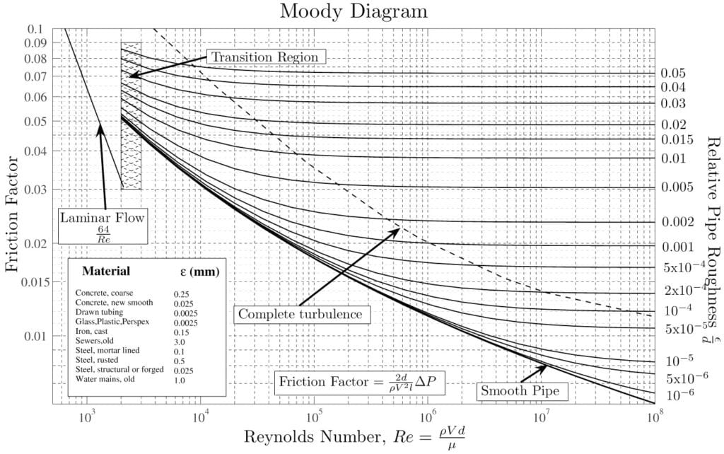
An example is a flow in a closed pipe, studied analytically through the Moody’s chart (Figure 3). The behavior of the flow (described through the friction factor) depends both on the Reynolds number and the relative roughness$^3$. The relative roughness is a “local” factor, which indicates the presence of a region that behaves differently because of its proximity to the boundary.

Shown on the left side, the laminar regime is linear and independent of the roughness.
Fully turbulent flows are on the right side of the chart (where the curve is flat) and occur at high Reynolds numbers and/or high values of roughness, which perturb the flow.
The most interesting part is the central one, the transition regime, in which the friction factor is highly dependent on both the Reynolds number and the relative roughness. Also, the description of the beginning of the turbulent regime is not reliable, because of its aleatory nature.

Moody Diagram showing change in friction factor with change in Reynolds number and relative roughness — Figure 3: Moody Diagram with the arrows distinguishing the flow regimes

Applications of Laminar Flow

Laminar flows have both academic and industrial applications.

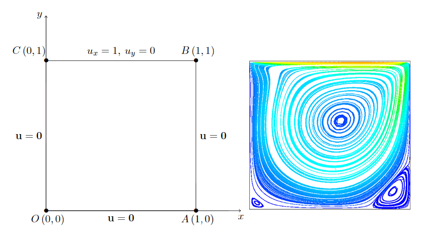
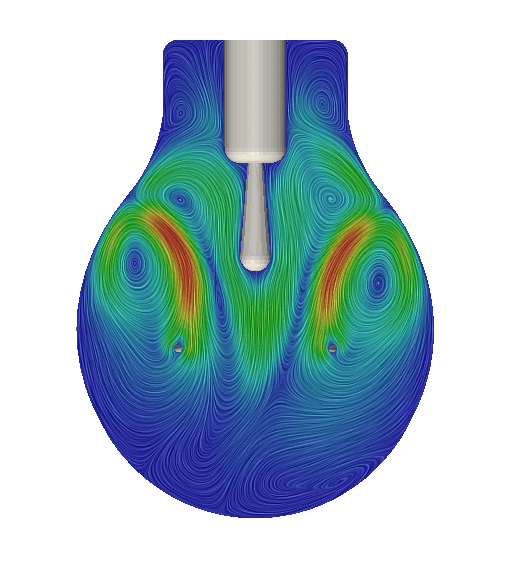
Many flows in the laminar regime are used as benchmarks for the development of advanced simulation techniques. This is the case of the “lid-driven cavity”$^4$, described in Figure 4(a), which shows a critical Reynolds number of $Re=1000$. The resulting velocity field (Figure 4(b)) depends on the Reynolds number, and the main flow characteristics (e.g. number of eddies, eddies center position, velocity profile) have been extensively benchmarked.

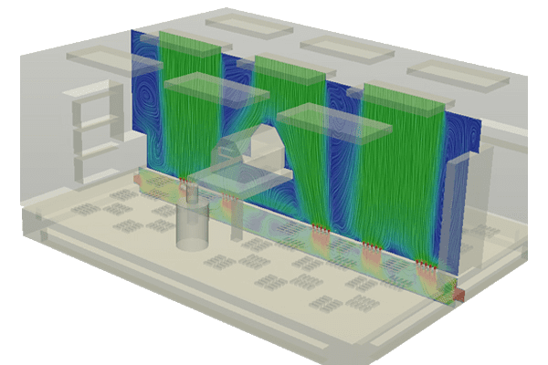
Lid-driven cavity with Geometry, boundary conditions and velocity streamlines for Reynolds number equal to 500 — Figure 4: Lid-driven cavity: (a) Geometry and boundary conditions where u=0 represents a wall; (b) Velocity Streamlines for Re=500 showing high velocity at the top (red) and almost zero velocity near the walls (blue)

From the industrial point of view, the laminar regime is usually developed in flows with low velocity, low density or high viscosity. This is usually the case with natural convection (Figure 5) or ventilation systems working at low velocities (Figure 6).

Simulation image showing laminar flows of natural convection inside a bulb — Figure 5: Natural convection inside a bulb where temperature difference regulates the laminar flow.

Streamlines showing ventilation inside a clean room flowing in a laminar regime — Figure 6: Ventilation system inside a cleanroom. Smooth continuous streamlines for low-velocity flows can be observed, governed by the temperature difference

References

“An experimental investigation of the circumstances which determine whether the motion of water shall be direct or sinuous, and of the law of resistance in parallel channels”. Proceedings of the Royal Society of London. 35 (224-226): 84–99
“Arnold Sommerfeld: Science, Life and Turbulent Times 1868-1951”, Michael Eckert. Springer Science Business Media, 24 giu 2013.
Moody, L. F. (1944), “Friction factors for pipe flow”, Transactions of the ASME, 66 (8): 671–684
C.T. Shin U. Ghia, K.N. Ghia. High-Resolution for incompressible flow using the Navier-Stokes equations and the multigrid method. J. Comput. Phys., 48:387–411, 1982.

Last updated: August 11th, 2023

Did this article solve your issue?

How can we do better?

We appreciate and value your feedback.

What's Next

What is Turbulent Flow?

Problem Configuration	Laminar regime	Transition regime	Turbulent Regime
Flow around a foil parallel to the main flow	\(Re<5\cdot 10^5\)	\(5\cdot 10^5 < Re < 10^7\)	\(Re > 10^7\)
Flow around a cylinder whose axis is perpendicular to the main flow	\(Re < 2 \cdot 10^5\)	\(Re \cong 2 \cdot 10^5\)	\(Re > 2\cdot 10^5\)
Flow around a sphere	\(Re < 2 \cdot 10^5\)	\(Re \cong 2 \cdot 10^5\)	\(Re > 2\cdot 10^5\)
Flow inside a circular-section pipe	\(Re < 2300\)	\(2300 < Re < 4000\)	\(Re > 4000\)