Creep

Creep is the inelastic, irreversible deformation of solid materials during time. It is a life limiting factor for a structure and depends on variables such as stress, strain, temperature and time. This dependency can be modeled as followed:

$$ \begin{equation}\label{creep_dependency_eq}
\dot{\mathbf{\epsilon}}_{cr} = f(\sigma,\epsilon,T,t) \end{equation} \tag1$$

Creep can occur in all crystalline materials, such as metal or glass. It has various impacts on the behavior of the material, and can ultimately lead to the following problems: [NAFEMS_HT21]

1. Disproportionate deformation leads to buckling or failure. In machines with moving parts this can reduce the size of gaps and lead to frictional abrasion.
2. The connection of bolted parts can loosen over time, because of relaxations of the pre-stressing. This relaxation can also occur in cables, gaskets, and flanges.
3. Excessive heat and load cycles can favor the propagation of cracks, which can lead to damage and ultimately to failure of the part.

Because of these extremely different factors, the effects of creep in certain situations can be highly complex. By undertaking creep analysis the influence of these effects can be evaluated and the lifetime of parts can be estimated. Especially, in the hot section of turbines of commercial and military plants, this can be a crucial factor for the design process and optimization costs.

Three Stages of Creep

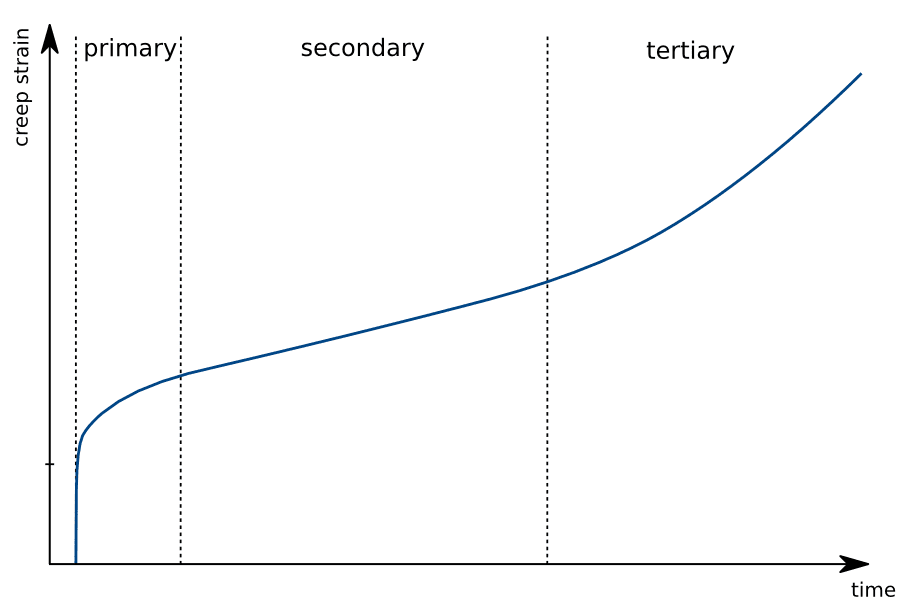
Creep can be divided into three different stages: primary creep, secondary creep and tertiary creep:

Primary creep (\(-1 < m < 0\)) starts rapidly with an infinite creep rate at the initialization. Here, \(m\) is the time index (for the strain rate form of the equations). It occurs after a certain amount of time and slows down constantly. It lasts for the first hour after applying the load and is essential in calculating the relaxation over time.

Secondary creep (\(m = 0\)) follows right after the primary creep stage. The strain rate is now constant over a long period of time.

The strain rate in the tertiary creep stage is growing rapidly until failure. This happens in a short period of time and is not of great interest. Therefore, only primary and secondary creep are modeled on the SimScale platform.

Calculating the Creep Strain

The creep strain equations are based on an additive strain decomposition:

$$ \begin{equation}\label{strain_decomposition}
\mathbf{\epsilon}_{tot} = \mathbf{\epsilon}_{el} + \mathbf{\epsilon}_{pl} + \mathbf{\epsilon}_{cr} \end{equation} $$

$$ \begin{equation}\label{small_strain_hypo} \mathbf{\sigma} = \mathbf{D} : \mathbf{\epsilon}_{el} \end{equation} $$

$$ \begin{equation}\label{creep_strain_eq} \dot{\mathbf{\epsilon}}_{cr} = \frac{3}{2} \dot{\epsilon^c} \frac {\tilde{\mathbf{\sigma}}}{\sigma_{eq}} \end{equation} $$

Where:

• \(\mathbf{\epsilon}_{tot}\) : total strain tensor
• \(\mathbf{\epsilon}_{el}\) : elastic strain tensor
• \(\mathbf{\epsilon}_{pl}\) : plastic strain tensor
• \(\mathbf{\epsilon}_{cr}\) : creep strain tensor
• \(\mathbf{\epsilon^c}\) : equivalent creep strain
• \(\tilde{\mathbf{\sigma}}\) : deviatoric stress tensor
• \(\sigma_{eq}\) : equivalent stress
• \(\mathbf{D}\) : elasticity tensor
• The dot over a quantity represents the rate of change, e.g., the creep tensor strain rate \( \dot{ \epsilon }_{cr} \)

The elastic strain \(\mathbf{\epsilon}_{el}\) occurs right after applying the load and is connected with the stresses through the elasticity tensor \(\mathbf{D}\) in equation 1. The plastic strain \(\mathbf{\epsilon}_{pl}\) results from excessive loading and is irreversible. The creep strain tensor can be calculated with the equivalent creep strain \(\mathbf{\epsilon^c}\), the deviatoric stress \(\tilde{\mathbf{\sigma}}\) and the equivalent stress \(\sigma_{eq}\). The deviatoric stress \(\tilde{\mathbf{\sigma}}\) causes distortion of the body and results after splitting the stress tensor in additive isotropic and deviatoric components.

Calculating the Equivalent Creep Strain

The fundamental creep law type defined as creep strain rate equation is available in SimScale:

Power or Bailey-Norton Law:

$$ \dot{\epsilon^c} = A \cdot \sigma^{n} \cdot t^m \cdot \epsilon^{k}$$

where we have

• \(A\): a constant, which depends on problem
• \(n\): creep stress index, \(1 <= n <= 10\)
• \(m\): time index, \(-1 < m <= 0\)
• \(k\): creep strain index

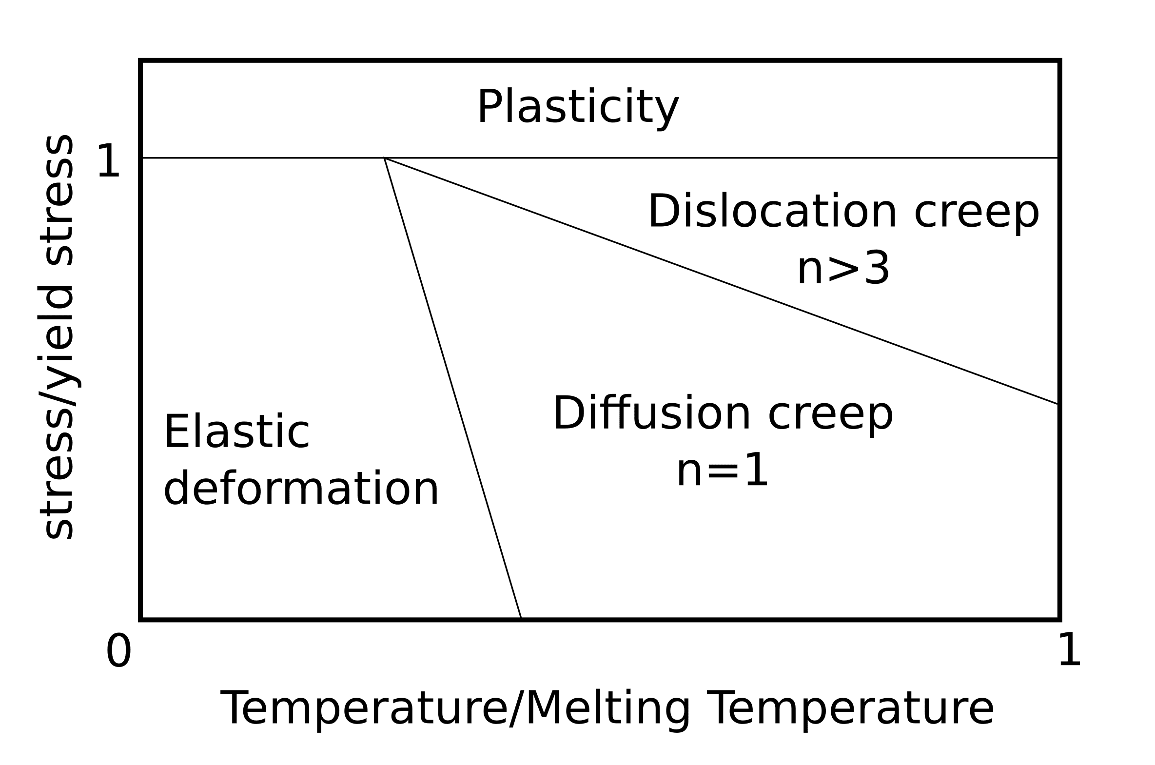
The creep stress index depends on the temperature and the stress level and can be determined with the help of an Ashby deformation mechanism map.

On the basis of these basic laws, three different creep formulations are currently available on the platform:

Norton (Power Law)

In this formulation, the creep strain rate only depends on the stresses. Therefore \(m\) and \(k\) are equal to zero:

$$ \dot{\epsilon^c} = A \cdot \sigma^{n}$$

Time Hardening (Power Law)

In this formulation, the creep strain rate depends also on time:

$$ \dot{\epsilon^c} = A \cdot \sigma^{n} \cdot t^m$$

Strain Hardening (Power Law)

In this formulation, the creep strain rate depends on the stresses and the creep strains. (For convenience \(k\) is referred to as \(m\) on the platform.)

$$ \dot{\epsilon^c} = A \cdot \sigma^{n} \cdot (\epsilon^c)^k$$

Defining Creep Materials in SimScale

Creep behavior can be applied to Linear Elastic and Elasto-Plastic material models. To define the model, follow the steps given below:

• Navigate to the Materials tab, in the simulation tree. Check that the Material behavior is Linear Elastic or Elasto-plastic.
• Select the appropriate Creep formulation for the problem.
• Input the \( A, N, M \) parameters according to the selected formulation.

Important Remarks

1. The creep formulation parameters \((A, m, n)\) and \((\epsilon_0^c, \sigma_0)\) are defined in the sense of the above equations with respect to the rate form of the creep laws.

2. It is important to have a consistent unit system when converting parameters found in literature or material supplier or test data. Often the creep parameters are given related to length measure in \(mm\), stresses in \(MPa\), and time in hours. An example of how to convert the parameter \(A\) of the Time Hardening or Strain Hardening formulation would be: \(A_{SI} = \frac{1}{3600} \cdot \frac{1}{3600^m} \cdot \frac{1}{10^{6n}} \cdot A_{MPa\;h}\)

3. Especially when primary creep is observed it is very important to refine the time-stepping sufficiently to capture the creep behavior correctly. Therefore it is advised to use the Field change criteria of the automatic time stepping available for Code_Aster.

Related Projects

• Validation case: 3D Triaxial Load Secondary Creep (NAFEMS Test 6(a))
• Validation case: 3D Triaxial Displacement Secondary Creep (NAFEMS Test 6(b))
• Validation case: 3D Triaxial Load Primary Creep (NAFEMS Test 11)

Last updated: March 7th, 2024